2.1 Machine learning lecture 2 course notes  (Page 2/6)

In the equation above, “ $|\Sigma |$ ” denotes the determinant of the matrix $\Sigma$ .

For a random variable $X$ distributed $\mathcal{N}(\mu ,\Sigma )$ , the mean is (unsurprisingly) given by $\mu$ :

The covariance of a vector-valued random variable $Z$ is defined as $\mathrm{Cov}\left(Z\right)=\mathrm{E}\left[(Z-\mathrm{E}\left[Z\right]){(Z-\mathrm{E}\left[Z\right])}^T\right]$ . This generalizes the notion of the variance of a real-valued random variable. The covariance canalso be defined as $\mathrm{Cov}\left(Z\right)=\mathrm{E}\left[Z{Z}^T\right]-\left(\mathrm{E}\left[Z\right]\right){\left(\mathrm{E}\left[Z\right]\right)}^T$ . (You should be able to prove to yourself that these two definitions are equivalent.)If $X\sim \mathcal{N}(\mu ,\Sigma )$ , then

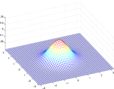
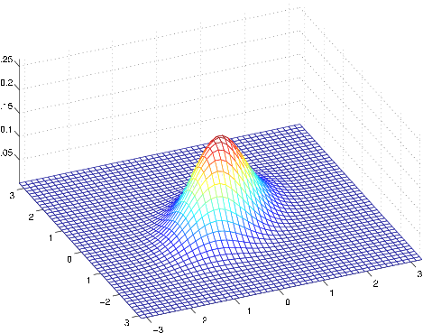
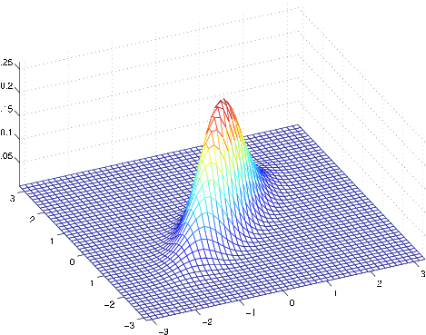
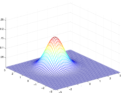
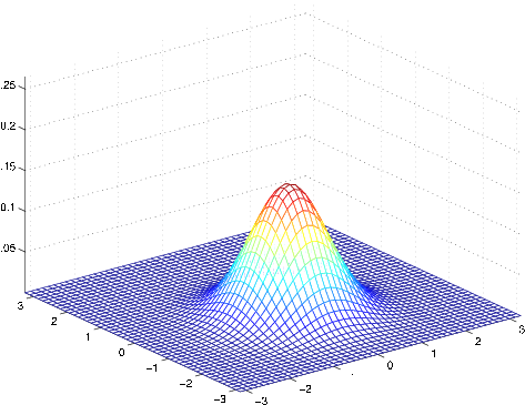
Here're some examples of what the density of a Gaussian distribution looks like:

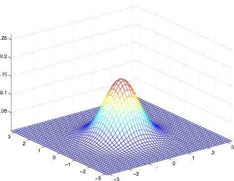
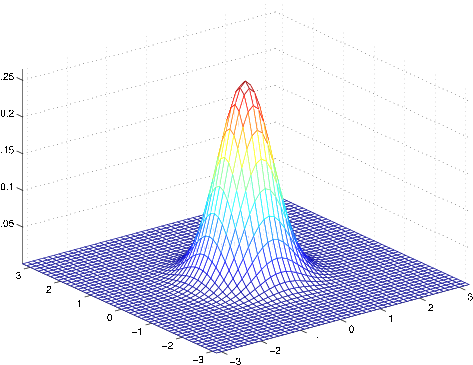
The left-most figure shows a Gaussian with mean zero (that is, the 2x1 zero-vector) and covariance matrix $\Sigma =I$ (the 2x2 identity matrix). A Gaussian with zero mean and identity covariance is also called the standard normal distribution . The middle figure shows the density of a Gaussian with zero mean and $\Sigma =0.6I$ ; and in the rightmost figure shows one with , $\Sigma =2I$ . We see that as $\Sigma$ becomes larger, the Gaussian becomes more “spread-out,” and as it becomes smaller, the distribution becomesmore “compressed.”

Let's look at some more examples.

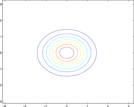
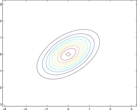
The figures above show Gaussians with mean 0, and with covariance matrices respectively

The leftmost figure shows the familiar standard normal distribution, and we see that as we increase the off-diagonal entry in $\Sigma$ , the density becomes more “compressed” towards the ${45}^{\circ }$ line (given by $x_1=x_2$ ). We can see this more clearly when we look at the contours of the same three densities:

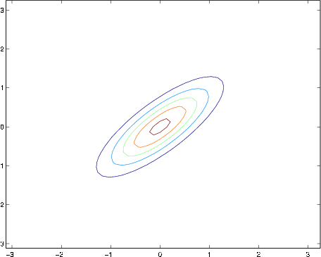
Here's one last set of examples generated by varying $\Sigma$ :

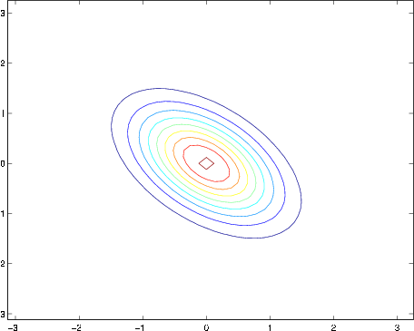
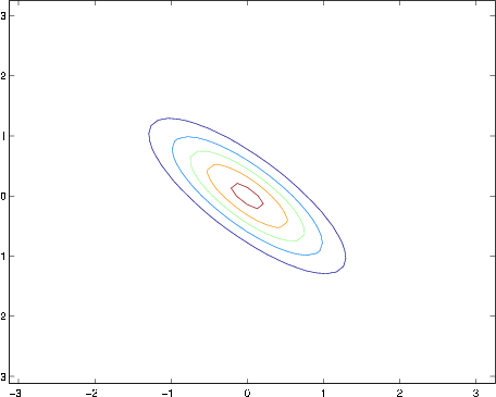
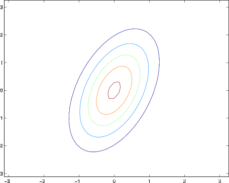
The plots above used, respectively,

From the leftmost and middle figures, we see that by decreasing the diagonal elements of the covariance matrix, the density now becomes “compressed” again, but in the opposite direction.Lastly, as we vary the parameters, more generally the contours will form ellipses (the rightmost figure showing an example).

As our last set of examples, fixing $\Sigma =I$ , by varying $\mu$ , we can also move the mean of the density around.

The figures above were generated using $\Sigma =I$ , and respectively

The gaussian discriminant analysis model

When we have a classification problem in which the input features $x$ are continuous-valued random variables, we can then use the Gaussian Discriminant Analysis (GDA) model, whichmodels $p\left(x\right|y)$ using a multivariate normal distribution. The model is:

Writing out the distributions, this is:

Here, the parameters of our model are $\Phi$ , $\Sigma$ , ${\mu }_0$ and ${\mu }_1$ . (Note that while there're two different mean vectors ${\mu }_0$ and ${\mu }_1$ , this model is usually applied using only one covariance matrix $\Sigma$ .) The log-likelihood of the data is given by

By maximizing $\ell$ with respect to the parameters, we find the maximum likelihood estimate of the parameters (see problem set 1) to be: