<< Chapter < Page Chapter >> Page >

Front Panel of CTFT and Its Properties: Combination of Input Signals Tab

Varying pulse width

Keep the default values of Time shift (=0) and Time scaling (=1) and vary the Pulse width of the rectangular pulse. First, set the value of the Pulse width to its minimum value (=0.01) and then increase it. Observe that increasing the Pulse width in the time domain decrements the width in the frequency domain (see [link] ). When the Pulse width is set to its maximum value (=1) in the frequency domain, only one value can be seen at the center frequency indicating the signal is of DC type (refer to Properties of CTFT section of Chapter 5).

Magnitude Spectrum for Different Pulse Widths: (a) 0.01, (b) 0.2, (c) 0.5, (d) 1

Time shift

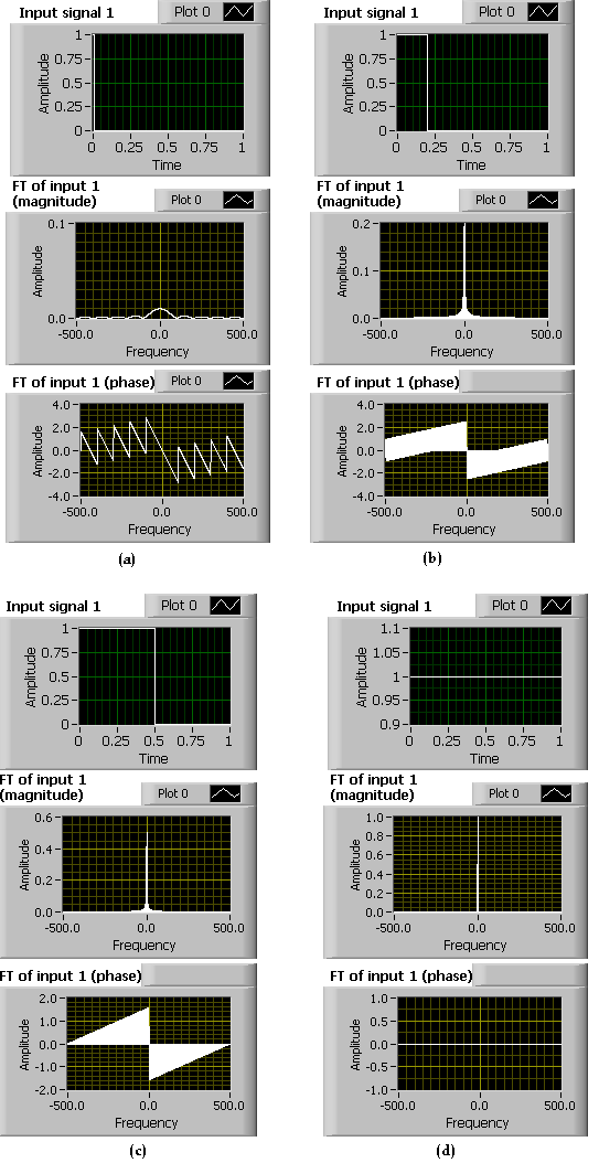
Next, for a fixed pulse width, vary the time shift. Observe that the phase spectrum changes but the magnitude spectrum remains the same. If the signal x ( t ) size 12{x \( t \) } {} is shifted by a constant t 0 size 12{t rSub { size 8{0} } } {} , its FT magnitude does not change, but the term ωt 0 size 12{ - ωt rSub { size 8{0} } } {} gets added to its phase angle. This verifies the time-shifting property of FT as stated in Properties of CTFT section of Chapter 5 (see [link] ).

Magnitude and Phase Spectrum for Different Time Shifts: (a) 0, (b) 0.2, (c) 0.5, (d) 0.7

Time scaling

Observe that increasing the control Time scaling makes the spectrum wider. This indicates that compressing the signal in the time domain leads to expansion in the frequency domain. This verifies the time-scaling property of FT as stated in Properties of CTFT section of Chapter 5 (see [link] ).

Magnitude Spectrum for Different Time Scalings: (a) 1, (b) 2, (c) 3, (d) 4

Linearity

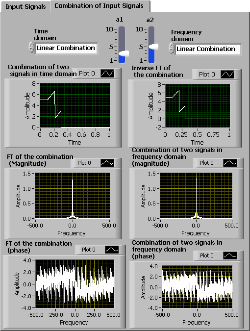
Here, combine two signals to examine the linearity property of FT. Select Linear Combination for the Time domain and Frequency domain combination method. This selection combines two time signals, x 1 ( t ) size 12{x rSub { size 8{1} } \( t \) } {} and x 2 ( t ) size 12{x rSub { size 8{2} } \( t \) } {} , linearly with the scaling factors, a 1 size 12{a rSub { size 8{1} } } {} and a 2 size 12{a rSub { size 8{2} } } {} , producing a new signal, a 1 x 1 ( t ) + a 2 x 2 ( t ) size 12{a rSub { size 8{1} } x rSub { size 8{1} } \( t \) +a rSub { size 8{2} } x rSub { size 8{2} } \( t \) } {} . [link] displays the FT of this linear combination. The linear combination in the frequency domain produces a new signal, a 1 X 1 ( ω ) + a 2 X 2 ( ω ) size 12{a rSub { size 8{1} } X rSub { size 8{1} } \( ω \) +a rSub { size 8{2} } X rSub { size 8{2} } \( ω \) } {} . [link] also displays the inverse FT of this combination. Observe that both combinations produce the same result in the time and frequency domains, as indicated by the linearity property stated in Properties of CTFT section of Chapter 5.

Verifying the Linearity Property of CTFT

Time convolution

In this part, convolve two signals in the time domain to examine the time-convolution property of FT. Select Convolution for Time domain and Multiplication for Frequency domain. This selection produces and displays a new signal, x 1 ( t ) x 2 ( t ) size 12{x rSub { size 8{1} } \( t \) * x rSub { size 8{2} } \( t \) } {} , by convolving the two time signals x 1 ( t ) size 12{x rSub { size 8{1} } \( t \) } {} and x 2 ( t ) size 12{x rSub { size 8{2} } \( t \) } {} . Multiplication in the frequency domain produces a new signal, X 1 ( ω ) X 2 ( ω ) size 12{X rSub { size 8{1} } \( ω \) X rSub { size 8{2} } \( ω \) } {} . The inverse FT of this multiplied signal is also displayed on the right. Note that both combinations produce the same outcome in the time and frequency domains. This verifies the time-convolution property stated in the Properties of CTFT section of Chapter 5 (see [link] ).

Verifying the Time-Convolution Property of CTFT

Frequency convolution

Convolve two signals in the frequency domain to examine the frequency-convolution property of FT. Select Convolution for Frequency domain and Multiplication for Time domain. This selection convolves the two time signals X 1 ( ω ) size 12{X rSub { size 8{1} } \( ω \) } {} and X 2 ( ω ) size 12{X rSub { size 8{2} } \( ω \) } {} to produce a new signal, X 1 ( ω ) X 2 ( ω ) size 12{X rSub { size 8{1} } \( ω \) * X rSub { size 8{2} } \( ω \) } {} . The inverse FT of the convolved signal is displayed. Multiplication in Time domain produces a new signal, x 1 ( t ) x 2 ( t ) size 12{x rSub { size 8{1} } \( t \) x rSub { size 8{2} } \( t \) } {} . The FT of this multiplied signal is also displayed. Note that both combinations produce the same outcome in the time and frequency domains. This verifies the frequency-convolution property stated in the Properties of CTFT section of Chapter 5 (see [link] ).

Questions & Answers

differentiate between demand and supply giving examples
Lambiv Reply
differentiated between demand and supply using examples
Lambiv
what is labour ?
Lambiv
how will I do?
Venny Reply
how is the graph works?I don't fully understand
Rezat Reply
information
Eliyee
devaluation
Eliyee
t
WARKISA
hi guys good evening to all
Lambiv
multiple choice question
Aster Reply
appreciation
Eliyee
explain perfect market
Lindiwe Reply
In economics, a perfect market refers to a theoretical construct where all participants have perfect information, goods are homogenous, there are no barriers to entry or exit, and prices are determined solely by supply and demand. It's an idealized model used for analysis,
Ezea
What is ceteris paribus?
Shukri Reply
other things being equal
AI-Robot
When MP₁ becomes negative, TP start to decline. Extuples Suppose that the short-run production function of certain cut-flower firm is given by: Q=4KL-0.6K2 - 0.112 • Where is quantity of cut flower produced, I is labour input and K is fixed capital input (K-5). Determine the average product of lab
Kelo
Extuples Suppose that the short-run production function of certain cut-flower firm is given by: Q=4KL-0.6K2 - 0.112 • Where is quantity of cut flower produced, I is labour input and K is fixed capital input (K-5). Determine the average product of labour (APL) and marginal product of labour (MPL)
Kelo
yes,thank you
Shukri
Can I ask you other question?
Shukri
what is monopoly mean?
Habtamu Reply
What is different between quantity demand and demand?
Shukri Reply
Quantity demanded refers to the specific amount of a good or service that consumers are willing and able to purchase at a give price and within a specific time period. Demand, on the other hand, is a broader concept that encompasses the entire relationship between price and quantity demanded
Ezea
ok
Shukri
how do you save a country economic situation when it's falling apart
Lilia Reply
what is the difference between economic growth and development
Fiker Reply
Economic growth as an increase in the production and consumption of goods and services within an economy.but Economic development as a broader concept that encompasses not only economic growth but also social & human well being.
Shukri
production function means
Jabir
What do you think is more important to focus on when considering inequality ?
Abdisa Reply
any question about economics?
Awais Reply
sir...I just want to ask one question... Define the term contract curve? if you are free please help me to find this answer 🙏
Asui
it is a curve that we get after connecting the pareto optimal combinations of two consumers after their mutually beneficial trade offs
Awais
thank you so much 👍 sir
Asui
In economics, the contract curve refers to the set of points in an Edgeworth box diagram where both parties involved in a trade cannot be made better off without making one of them worse off. It represents the Pareto efficient allocations of goods between two individuals or entities, where neither p
Cornelius
In economics, the contract curve refers to the set of points in an Edgeworth box diagram where both parties involved in a trade cannot be made better off without making one of them worse off. It represents the Pareto efficient allocations of goods between two individuals or entities,
Cornelius
Suppose a consumer consuming two commodities X and Y has The following utility function u=X0.4 Y0.6. If the price of the X and Y are 2 and 3 respectively and income Constraint is birr 50. A,Calculate quantities of x and y which maximize utility. B,Calculate value of Lagrange multiplier. C,Calculate quantities of X and Y consumed with a given price. D,alculate optimum level of output .
Feyisa Reply
Answer
Feyisa
c
Jabir
the market for lemon has 10 potential consumers, each having an individual demand curve p=101-10Qi, where p is price in dollar's per cup and Qi is the number of cups demanded per week by the i th consumer.Find the market demand curve using algebra. Draw an individual demand curve and the market dema
Gsbwnw Reply
suppose the production function is given by ( L, K)=L¼K¾.assuming capital is fixed find APL and MPL. consider the following short run production function:Q=6L²-0.4L³ a) find the value of L that maximizes output b)find the value of L that maximizes marginal product
Abdureman
types of unemployment
Yomi Reply
What is the difference between perfect competition and monopolistic competition?
Mohammed
Got questions? Join the online conversation and get instant answers!
Jobilize.com Reply

Get Jobilize Job Search Mobile App in your pocket Now!

Get it on Google Play Download on the App Store Now


Source:  OpenStax, An interactive approach to signals and systems laboratory. OpenStax CNX. Sep 06, 2012 Download for free at http://cnx.org/content/col10667/1.14
Google Play and the Google Play logo are trademarks of Google Inc.

Notification Switch

Would you like to follow the 'An interactive approach to signals and systems laboratory' conversation and receive update notifications?

Ask