0.13 Lecture 14:the laplace transform - method of solution

Lecture #14:

THE LAPLACE TRANSFORM - METHOD OF SOLUTION

Motivation:

• Continue to describe methods for representing signals as superpositions of complex exponential functions
• Develop efficient methods for analyzing LTI systems

Outline:

• Review of last lecture

• Laplace transform of the family of singularity functions

• More on the region of convergence

• Analysis of networks with the Laplace transform — the impedance method

• Finding inverse transforms — partial fraction expansion

• Conclusion

• Historical perspective — Oliver Heaviside

Review

• The Laplace transform represents a time function as a superposition of complex exponentials.

• A time function is related uniquely to a Laplace transform if the ROC is specified.

• If the Laplace transform of a sum of causal and anti-causal exponential time functions exists, its ROC is a strip in the s-plane parallel to the jω-axis.

I. LAPLACE TRANSFORMS OF SINGULARITY FUNCTIONS

1/ Unit impulse function

$L\{\delta (t)\}=\underset{-\infty }{\overset{\infty }{\int }}\delta (t)e^{-\text{st}}\text{dt}$

Recall the definition of the unit impulse

$\underset{-\infty }{\overset{\infty }{\int }}\delta (t)f(t)\text{dt}=f(0)$

Hence,

$L\{\delta (t)\}=1$

for all values of s. The region of convergence is the entire s plane.

2/ Unit impulse function delayed — use of properties

The Laplace transform of an impulse located at t = 0 is

$L\{\delta (t)\}=1$

Using the delay property,

$\begin{array}{}x(t)\begin{array}{cc}& \end{array}\stackrel{L}{\iff }\begin{array}{cc}& \end{array}X(s)\\ x(t-T)\begin{array}{cc}& \end{array}\stackrel{L}{\iff }\begin{array}{cc}& \end{array}X(s)e^{-\text{sT}}\end{array}$

the Laplace transform of the delayed impulse is

$L\{\delta (t-T)\}=e^{-\text{sT}}$

and the region of convergence is the whole s plane.

Two-minute miniquiz problem

Problem 5-1

Find the Laplace transform including the ROC for

$x(t)=e^{-2(t-4)}u(t-4)$

Solution

We use the Laplace transform of the causal exponential time function and time delay property to solve this problem.

$\begin{array}{}{e}^{-\mathrm{2t}}u(t)\begin{array}{cc}& \end{array}\stackrel{L}{\iff }\begin{array}{cc}& \end{array}\frac{1}{s+2}\begin{array}{cc}& \end{array}\text{for}\begin{array}{cc}& \end{array}\sigma >-2\\ e^{-2(t-4)}u(t-4)\begin{array}{cc}& \end{array}\stackrel{L}{\iff }\begin{array}{cc}& \end{array}\frac{1}{s+2}{e}^{-\mathrm{4s}}\begin{array}{cc}& \end{array}\text{for}\begin{array}{cc}& \end{array}\sigma >-2\end{array}$

3/ Singularity functions and their relatives

The Laplace transform of a unit impulse is

$\delta (t)\begin{array}{cc}& \end{array}\stackrel{L}{\iff }\begin{array}{cc}& \end{array}1\begin{array}{cc}& \end{array}\text{for}\begin{array}{cc}& \end{array}\text{all}\begin{array}{cc}& \end{array}s$

and from the Laplace transform of a causal exponential with α = 0 we have the Laplace transform of a causal step function

$u(t)\begin{array}{cc}& \end{array}\stackrel{L}{\iff }\begin{array}{cc}& \end{array}\frac{1}{s}\begin{array}{cc}& \end{array}\text{for}\begin{array}{cc}& \end{array}\sigma >0$

Note this fits together with the time differentiation property

$\frac{\text{dx}(t)}{\text{dt}}\stackrel{}{\begin{array}{cc}& \end{array}\stackrel{L}{\iff }}\begin{array}{cc}& \end{array}\text{sX}(s)$

since in a generalized function sense

$\delta (t)=\frac{\text{du}(t)}{\text{dt}}\begin{array}{cc}& \end{array}\stackrel{L}{\iff }\begin{array}{cc}& \end{array}L\{\delta (t)\}=s\left[\frac{1}{s}\right]=1$

We use the multiplication by t property

$\text{tx}(t)\begin{array}{cc}& \end{array}\stackrel{L}{\iff }\begin{array}{cc}& \end{array}-\frac{\text{dX}(s)}{\text{ds}}$

to obtain

$\text{tu}(t)\begin{array}{cc}& \end{array}\stackrel{L}{\iff }\begin{array}{cc}& \end{array}-\frac{d}{\text{ds}}\left[\frac{1}{s}\right]=\frac{1}{s^2}\begin{array}{cc}& \end{array}\text{for}\begin{array}{cc}& \end{array}\sigma >0$

and use it again to obtain

$t^{2}u(t)\begin{array}{cc}& \end{array}\stackrel{L}{\iff }\begin{array}{cc}& \end{array}-\frac{d}{\text{ds}}\left[\frac{1}{s^2}\right]=\frac{1}{s^3}\begin{array}{cc}& \end{array}\text{for}\begin{array}{cc}& \end{array}\sigma >0$

which implies that by induction

$t^{n}u(t)\begin{array}{cc}& \end{array}\stackrel{L}{\iff }\begin{array}{cc}& \end{array}\frac{n!}{s^{n+1}}\begin{array}{cc}& \end{array}\text{for}\begin{array}{cc}& \end{array}\sigma >0$

or

$\frac{t^{n-1}}{(n-1)!}u(t)\begin{array}{cc}& \end{array}\stackrel{L}{\iff }\begin{array}{cc}& \end{array}\frac{1}{s^n}\begin{array}{cc}& \end{array}\text{for}\begin{array}{cc}& \end{array}\sigma >0$

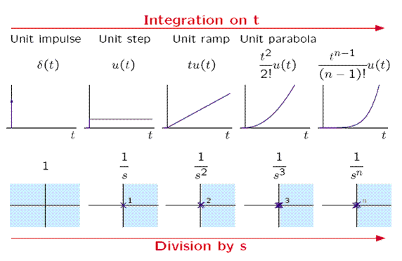
4/ Summary of singularity functions and their relatives

5/ Wild and crazy singularity functions

Since taking the derivative of a time function corresponds to multiplying the Laplace transform by s we can contemplate the derivative of the unit impulse called the unit doublet.

$\frac{\mathrm{d\delta }(t)}{\text{dt}}=\stackrel{\text{.}}{\delta }(t)\begin{array}{cc}& \end{array}\stackrel{L}{\iff }\begin{array}{cc}& \end{array}s$

This process can be continued by taking successive derivatives of the impulse to form the unit triplet which has Laplace transform $s^2$ , unit quadruplet, etc. In general, the nth derivative of the unit impulse has a Laplace transform $s^n$ . We shall consider the usefulness of these higher order singularity functions later!