Method for representing DT signals as superpositions of complex geometric (exponential) functions.
Lecture #15:
THE BILATERAL Z-TRANSFORM
Motivation: Method for representing DT signals as superpositions of complex geometric (exponential) functions
Outline:
Review of last lecture
The bilateral Z-transform
– Definition
– Properties
Inventory of transform pairs
Conclusion
Review of last lecture
Solve linear difference equation for a causal exponential input
Solve homogeneous equation for n>0
Solve characteristic polynomial for λ.
Solve for a particular solution for n>0
Assuming
and solving for Y yields
Logic for an analysis method for DT LTI systems
characterizes system compute
efficiently.
In steady state, response to
is
.
Represent arbitrary x[n] as superpositions of
on z.
Compute response y[n] as superpositions of
on z.
I. THE BILATERAL Z-TRANSFORM
1/ Definition
The bilateral Z-transform is defined by the analysis formula
is defined for a region in z — called the region of convergence — for which the sum exists.
The inverse transform is defined by the synthesis formula
Since z is a complex quantity,
is a complex function of a complex variable. Hence, the synthesis formula involves integration in the complex z domain. We shall not perform this integration in this subject. The synthesis formula will be used only to prove theorems and not to compute time functions directly.
a/ Approach
An inventory of time functions and their Z-transforms will be developed by
Using the Z-transform properties,
Determining the Z-transforms of elementary DT time functions,
Combining the results of the above two items.
b/ Notation
We shall use two useful notations — Z{x[n]} signifies the Z-transform of x[n]and a Z-transform pair is indicated by
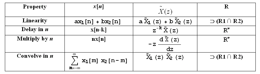
2/ Properties
a/ Linearity
The proof follows from the definition of the Z-transform as a sum.
b/ Delay by k
This result can be seen using the synthesis formula,
c/ Multiply by n
This result can be seen using the analysis formula.
Most proofs of Z-transform properties are simple. Some of the important properties are summarized here.
R, R1, and R2 are the ROCs of
,
, and
, respectively. * Exceptions may occur at z = 0 and z = ∞.
II. Z-TRANSFORMS OF SIMPLE TIME FUNCTIONS
1/ Unit sample function
The Z-transform of the unit sample is
for all values of z, i.e., the ROC is the entire z plane.
2/ Unit step function
The unit step and unit sample functions are simply related.