2.3 Machine learning lecture 4 course notes  (Page 5/5)

Let's put all this together into a theorem.

Theorem. Let $\left|\mathcal{H}\right|=k$ , and let any $m,\delta$ be fixed. Then with probability at least $1-\delta$ , we have that

This is proved by letting $\gamma$ equal the $\sqrt{·}$ term, using our previous argument that uniform convergence occurs with probability at least $1-\delta$ , and then noting that uniform convergence implies $\epsilon \left(h\right)$ is at most $2\gamma$ higher than $\epsilon \left(h^{*}\right)={min}_{h\in \mathcal{H}}\epsilon \left(h\right)$ (as we showed previously).

This also quantifies what we were saying previously saying about the bias/variance tradeoff in model selection. Specifically, suppose we have some hypothesis class $\mathcal{H}$ , and are considering switching to some much larger hypothesis class ${\mathcal{H}}^{\text{'}}\supseteq \mathcal{H}$ . If we switch to ${\mathcal{H}}^{\text{'}}$ , then the first term ${min}_h\epsilon \left(h\right)$ can only decrease (since we'd then be taking a min over a larger set of functions). Hence,by learning using a larger hypothesis class, our “bias” can only decrease. However, if k increases, then the second $2\sqrt{·}$ term would also increase. This increase corresponds to our “variance” increasingwhen we use a larger hypothesis class.

By holding $\gamma$ and $\delta$ fixed and solving for $m$ like we did before, we can also obtain the following sample complexity bound:

Corollary. Let $\left|\mathcal{H}\right|=k$ , and let any $\delta ,\gamma$ be fixed. Then for $\epsilon \left(\widehat{h}\right)\le {min}_{h\in \mathcal{H}}\epsilon \left(h\right)+2\gamma$ to hold with probability at least $1-\delta$ , it suffices that

The case of infinite $\mathcal{H}$

We have proved some useful theorems for the case of finite hypothesis classes. But many hypothesis classes, including any parameterized by real numbers(as in linear classification) actually contain an infinite number of functions. Can we prove similar results for this setting?

Let's start by going through something that is not the “right” argument. Better and more general arguments exist , but this will be useful for honing our intuitions about the domain.

Suppose we have an $\mathcal{H}$ that is parameterized by $d$ real numbers. Since we are using a computer to represent real numbers, and IEEE double-precision floating point ( double 's in C) uses 64 bitsto represent a floating point number, this means that our learning algorithm, assuming we're using double-precision floating point, is parameterized by $64d$ bits. Thus, our hypothesis class really consists of at most $k=2^{64d}$ different hypotheses. From the Corollary at the end of the previous section, we therefore find that, to guarantee $\epsilon \left(\widehat{h}\right)\le \epsilon \left(h^{*}\right)+2\gamma$ , with to hold with probability at least $1-\delta$ , it suffices that $m\ge O\left(\frac{1}{{\gamma }^2},log,\frac{2^{64d}}{\delta }\right)=O\left(\frac{d}{{\gamma }^2},log,\frac{1}{\delta }\right)=O_{\gamma ,\delta }\left(d\right)$ . (The $\gamma ,\delta$ subscripts are to indicate that the last big- $O$ is hiding constants that may depend on $\gamma$ and $\delta$ .) Thus, the number of training examples needed is at most linear in the parameters of the model.

The fact that we relied on 64-bit floating point makes this argument not entirely satisfying, but the conclusion is nonetheless roughly correct: If what we're going to do is try to minimize training error,then in order to learn “well” using a hypothesis class that has $d$ parameters, generally we're going to need on the order of a linear number of training examples in $d$ .

(At this point, it's worth noting that these results were proved for an algorithm that uses empirical risk minimization. Thus, while the linear dependence of samplecomplexity on $d$ does generally hold for most discriminative learning algorithms that try to minimize trainingerror or some approximation to training error, these conclusions do not always apply as readily to discriminative learning algorithms. Giving good theoreticalguarantees on many non-ERM learning algorithms is still an area of active research.)

The other part of our previous argument that's slightly unsatisfying is that it relies on the parameterization of $\mathcal{H}$ . Intuitively, this doesn't seem like it should matter: We had written the classof linear classifiers as $h_{\theta }\left(x\right)=1\{{\theta }_0+{\theta }_1{x}_1+\cdots {\theta }_n{x}_n\ge 0\}$ , with $n+1$ parameters ${\theta }_0,...,{\theta }_n$ . But it could also be written $h_{u,v}\left(x\right)=1\{(u_0^2-v_0^2)+(u_1^2-v_1^2)x_1+\cdots (u_n^2-v_n^2)x_n\ge 0\}$ with $2n+2$ parameters $u_i,v_i$ . Yet, both of these are just defining the same $\mathcal{H}$ : The set of linear classifiers in $n$ dimensions.

To derive a more satisfying argument, let's define a few more things.

Given a set $S=\{x^{\left(i\right)},...,x^{\left(d\right)}\}$ (no relation to the training set) of points $x^{\left(i\right)}\in \mathcal{X}$ , we say that $\mathcal{H}$ shatters $S$ if $\mathcal{H}$ can realize any labeling on $S$ . I.e., if for any set of labels $\{y^{\left(1\right)},...,y^{\left(d\right)}\}$ , there existssome $h\in \mathcal{H}$ so that $h\left(x^{\left(i\right)}\right)=y^{\left(i\right)}$ for all $i=1,...d$ .

Given a hypothesis class $\mathcal{H}$ , we then define its Vapnik-Chervonenkis dimension , written $\mathrm{VC}\left(\mathcal{H}\right)$ , to be the size of the largest set that is shattered by $\mathcal{H}$ . (If $\mathcal{H}$ can shatter arbitrarily large sets, then $\mathrm{VC}\left(\mathcal{H}\right)=\infty$ .)

For instance, consider the following set of three points:

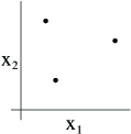
Can the set $\mathcal{H}$ of linear classifiers in two dimensions ( $h\left(x\right)=1\{{\theta }_0+{\theta }_1{x}_1+{\theta }_2{x}_2\ge 0\}$ ) can shatter the set above? The answer is yes. Specifically, we see that, for any of the eight possiblelabelings of these points, we can find a linear classifier that obtains “zero training error” on them:

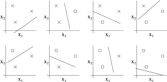
Moreover, it is possible to show that there is no set of 4 points that this hypothesis class can shatter. Thus, the largest set that $\mathcal{H}$ can shatter is of size 3, and hence $\mathrm{VC}\left(\mathcal{H}\right)=3$ .

Note that the VC dimension of $\mathcal{H}$ here is 3 even though there may be sets of size 3 that it cannot shatter. For instance, if we had a set of three pointslying in a straight line (left figure), then there is no way to find a linear separator for the labeling of the three points shown below (right figure):

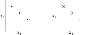
In order words, under the definition of the VC dimension, in order to prove that $\mathrm{VC}\left(\mathcal{H}\right)$ is at least $d$ , we need to show only that there's at least one set of size $d$ that $\mathcal{H}$ can shatter.

The following theorem, due to Vapnik, can then be shown. (This is, many would argue, the most important theorem in all of learning theory.)

Theorem. Let $\mathcal{H}$ be given, and let $d=\mathrm{VC}\left(\mathcal{H}\right)$ . Then with probability at least $1-\delta$ , we have that for all $h\in \mathcal{H}$ ,

Thus, with probability at least $1-\delta$ , we also have that:

In other words, if a hypothesis class has finite VC dimension, then uniform convergence occurs as $m$ becomes large. As before,this allows us to give a bound on $\epsilon \left(h\right)$ in terms of $\epsilon \left(h^{*}\right)$ . We also have the following corollary:

Corollary. For $|\epsilon \left(h\right)-\widehat{\epsilon }\left(h\right)|\le \gamma$ to hold for all $h\in \mathcal{H}$ (and hence $\epsilon \left(\widehat{h}\right)\le \epsilon \left(h^{*}\right)+2\gamma$ ) with probability at least $1-\delta$ , it suffices that $m=O_{\gamma ,\delta }\left(d\right)$ .

In other words, the number of training examples needed to learn “well” using $\mathcal{H}$ is linear in the VC dimension of $\mathcal{H}$ . It turns out that, for “most” hypothesis classes, the VC dimension (assuming a “reasonable” parameterization) is also roughly linear in the number of parameters.Putting these together, we conclude that (for an algorithm that tries to minimize training error) the number of trainingexamples needed is usually roughly linear in the number of parameters of $\mathcal{H}$ .