0.15 Lecture 16:the z transform - method of solution

Lecture #16:

THE Z-TRANSFORM –

METHOD OF SOLUTION

Motivation:

• Analysis of DT systems using the Z-transform
• Insight into numerical methods for solving differential equations

Outline:

• Review of last lecture

• Analysis of ladder network

• Analysis of discretized CT system

• Conclusion

Review of last lecture

The Z-transform is capable of representing a rich class of DT time functions. Z-transform pairs can be obtained by combining

• Z-transform properties

• The Z-transforms of elementary time functions

Logic for an analysis method for DT LTI systems

• $\stackrel{\text{~}}{H}(z)$ characterizes system $\Rightarrow$ compute $\stackrel{\text{~}}{H}(z)$ efficiently.
• In steady state, response to ${\text{Xz}}^n$ is $\stackrel{\text{~}}{H}(z)z^n$ .
• Represent arbitrary x[n] as superposition of $X(z)z^n$ on z.

• Compute response y[n] as superposition of $\stackrel{\text{~}}{H}(z)X(z)z^n$ on z.

We will analyze DT systems with the Z-transform method in a manner analogous to the use of the Laplace transform for CT systems.

I. OVERVIEW OF TRANSFORM METHOD OF SOLUTION

Electric ladder network

1/ Difference equation

We wish to find the unit sample response of an electric ladder network (considered in a previous lecture), i.e., we assume $v_i[n]=\delta [\nu ]$ .

As we found in a previous lecture, KCL at node n yields the difference equation

$-v_0[n+1]+(2+\alpha )v_0[n]-v_0[n-1]={\mathrm{\alpha v}}_i[n]\begin{array}{cc}& \end{array}\text{where}\begin{array}{cc}& \end{array}\alpha =\text{rg}$

2/ System function

We apply the Z-transform to the difference equation

${\text{-v}}_o[n+1]+(2+a){\text{v}}_o[n]{\text{-v}}_o[\text{n-1}]={\text{av}}_i[n]$ $$

to obtain

$(-z+(2+\alpha )-z^{-1}){\stackrel{\text{~}}{V}}_o(z)=\alpha {\stackrel{\text{~}}{V}}_i(z)$

so that

$\stackrel{\text{~}}{H}(z)=\frac{\stackrel{\text{~}}{V_o}(z)}{\stackrel{\text{~}}{V_i=}(z)}=\frac{-\mathrm{\alpha z}}{z^2-(2+\alpha )z+1}=\frac{-{\mathrm{\alpha z}}^{-1}}{1-(2+\alpha )z^{-1}+z^2}$

The z-form of the system function is easier for identifying the poles and zeros; the $z^{-1}$ -form is easier for calculating the inverse transform.

3/ Response

$v_i[n]=\delta [\nu ]$ implies that $\stackrel{\text{~}}{V_i}(z)=\text{1}$ with an ROC that is the whole z-plane. Therefore,

${\stackrel{\text{~}}{V}}_o(z)=\frac{-\mathrm{\alpha z}}{z^2-(2+\alpha )z+1}=\frac{-{\mathrm{\alpha z}}^{-1}}{1-(2+\alpha )z^{-1}+z^2}$

Thus, there is one zero and two poles. The poles are

$p_{\mathrm{1,2}}=\left[1+\frac{\alpha }{2}\right]\pm {\left[{\left[1+\frac{\alpha }{2}\right]}^2-1\right]}^{1/2}$

It is easy to show that $p_1{p}_2=1$ . Hence we write the poles as

$p_1=p=\left[1+\frac{\alpha }{2}\right]-{\left[{\left[1+\frac{\alpha }{2}\right]}^2-1\right]}^{1/2}\begin{array}{cc}& \end{array}\text{and}\begin{array}{cc}& \end{array}{p}_2=1/p_{1}1=1/p$

4/ Region of convergence

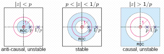
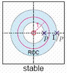
There are three possible ROCs for this response as shown below. On physical grounds, we expect the unit-sample response to be bounded.

Only the center ROC includes and unit circle and corresponds to a stable system.

Therefore, we conclude that

$$

where the pole at z = p contributes to the causal response while the pole at z = 1/p contributes to the anti-causal response.

5/ Inverse Z-transform

We perform a partial fraction expansion as follows

$\begin{array}{}{\stackrel{\text{~}}{V}}_o(z)=\frac{-{\mathrm{\alpha z}}^{-1}}{1-(2+\alpha )z^{-1}+z^2}=\frac{-{\mathrm{\alpha z}}^{-1}}{(1-p^{-1}{z}^{-1})(1-{\text{pz}}^{-1})}\\ \begin{array}{cc}& \end{array}=\frac{-(\mathrm{\alpha p})/(1-p^2)}{1-p^{-1}{z}^{-1}}+\frac{-({\mathrm{\alpha p}}^{-1})/(1-p^{-2})}{1-{\text{pz}}^{-1}}\end{array}$

which can be written as

${\stackrel{\text{~}}{V}}_o(z)=-\frac{\mathrm{\alpha p}}{1-p^2}\left[\frac{1}{1-p^{-1}{z}^{-1}}\right]+\frac{\mathrm{\alpha p}}{1-p^2}\left[\frac{1}{1-{\text{pz}}^{-1}}\right]$

Therefore,

$v_0[n]=\frac{\mathrm{\alpha p}}{1-p^2}{p}^{-n}u[-n-1]+\frac{\mathrm{\alpha p}}{1-p^2}{p}^{n}u[n]$

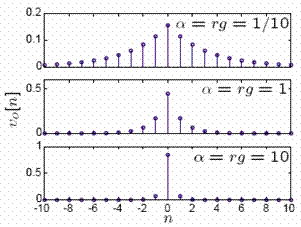
which can be written compactly as

$v_o[n]=\left[\frac{\mathrm{\alpha p}}{1-p^2}\right]p^{\mid n\mid }$

As the quantity α = rg increases, the spatial distribution of voltage gets narrower and narrower. Recall that r is the series resistance and g is the shunt conductance of the ladder.

II. DISCRETIZED CT SYSTEM

1/ Differential equation — RC Circuit

In a previous lecture, we considered the CT lowpass filter shown below.