| << Chapter < Page | Chapter >> Page > |
image(B);
colormap(gray(256));
axis('image');
The
image command works for both type
uint8 and
double images.
The
colormap command specifies the range of displayed gray levels,
assigning black to 0 and white to 255.It is important to note that if any pixel values are outside the range
0 to 255 (after processing), they will be clipped to 0 or 255 respectivelyin the displayed image.
It is also important to note that a floating point pixel value will berounded down ("floored") to an integer before it is displayed.
Therefore the maximum number of gray levels that will be displayed onthe monitor is 255, even if the image values take on a continuous range.
Now we will practice some simple operations on the yacht.tif image. Make a horizontally flipped version of the image by reversing theorder of each column. Similarly, create a vertically flipped image. Print your results.
Now, create a "negative" of the image by subtracting each pixel from 255 (here's an example of where conversion to double is necessary.) Print the result.
Finally, multiply each pixel of the original image by , and print the result.
Download the files house.tif and narrow.tif for the following sections.

The histogram of a digital image shows how its pixel intensities are distributed. The pixel intensities vary along the horizontal axis,and the number of pixels at each intensity is plotted vertically, usually as a bar graph.A typical histogram of an 8-bit image is shown in [link] .
Write a simple Matlab function
Hist(A) which will plot the histogram of image matrix
.
You may use Matlab's
hist function, however that function requires
a vector as input.An example of using
hist to plot a histogram of a matrix would be
x=reshape(A,1,M*N);
hist(x,0:255);
where
is an image, and
and
are the number of rows and columns in
.
The
reshape command is creating a row vector out of the image matrix,
and the
hist command plots a histogram with bins centered at
.
Download the image file
house.tif ,
and read it into Matlab.Test your
Hist function on the image. Label the axes of
the histogram and give it a title.

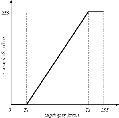
A pointwise transformation is a function that maps pixels from one intensity to another.An example is shown in [link] . The horizontal axis shows all possible intensitiesof the original image, and the vertical axis shows the intensities of the transformed image. This particular transformation maps the"darker" pixels in the range to a level of zero (black), and similarly maps the "lighter" pixels in to white. Then the pixels in the range are "stretched out" to use the full scale of . This can have the effect of increasing the contrast in an image.
Pointwise transformations will obviously affect the pixel distribution, hence they will change the shape of the histogram.If a pixel transformation can be described by a one-to-one function, , then it can be shown that the input and output histograms are approximately related by the following:

Notification Switch
Would you like to follow the 'Purdue digital signal processing labs (ece 438)' conversation and receive update notifications?