

| << Chapter < Page | Chapter >> Page > |
As we discussed in the previous section, exponential functions are used for many real-world applications such as finance, forensics, computer science, and most of the life sciences. Working with an equation that describes a real-world situation gives us a method for making predictions. Most of the time, however, the equation itself is not enough. We learn a lot about things by seeing their pictorial representations, and that is exactly why graphing exponential equations is a powerful tool. It gives us another layer of insight for predicting future events.
Before we begin graphing, it is helpful to review the behavior of exponential growth. Recall the table of values for a function of the form whose base is greater than one. We’ll use the function Observe how the output values in [link] change as the input increases by
Each output value is the product of the previous output and the base, We call the base the constant ratio . In fact, for any exponential function with the form is the constant ratio of the function. This means that as the input increases by 1, the output value will be the product of the base and the previous output, regardless of the value of
Notice from the table that
[link] shows the exponential growth function
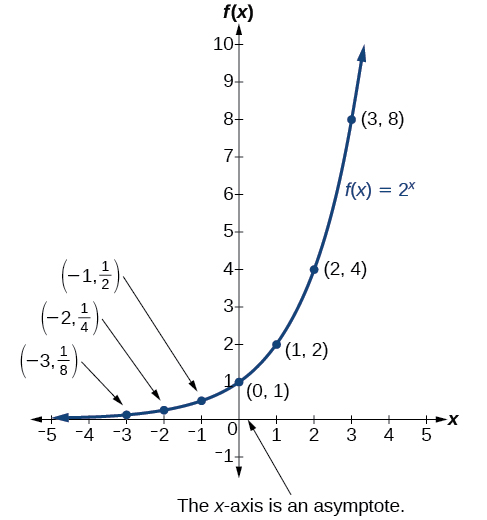
The domain of is all real numbers, the range is and the horizontal asymptote is
To get a sense of the behavior of exponential decay , we can create a table of values for a function of the form whose base is between zero and one. We’ll use the function Observe how the output values in [link] change as the input increases by
Again, because the input is increasing by 1, each output value is the product of the previous output and the base, or constant ratio
Notice from the table that
[link] shows the exponential decay function,
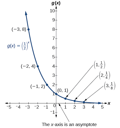
The domain of is all real numbers, the range is and the horizontal asymptote is
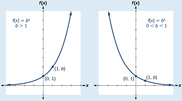
An exponential function with the form has these characteristics:
[link] compares the graphs of exponential growth and decay functions.
Given an exponential function of the form graph the function.
Notification Switch
Would you like to follow the 'Precalculus' conversation and receive update notifications?

|
|

|
|

|
|

|
|

|
|

|
|

|
|

|
|

|
|

|
|

|