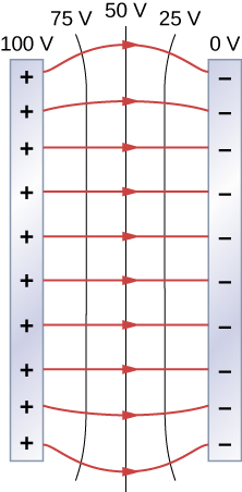
The electric field and equipotential lines between two metal plates. Note that the electric field is perpendicular to the equipotentials and hence normal to the plates at their surface as well as in the center of the region between them.
Consider the parallel plates in
[link] . These have equipotential lines that are parallel to the plates in the space between and evenly spaced. An example of this (with sample values) is given in
[link] . We could draw a similar set of equipotential isolines for gravity on the hill shown in
[link] . If the hill has any extent at the same slope, the isolines along that extent would be parallel to each other. Furthermore, in regions of constant slope, the isolines would be evenly spaced. An example of real topographic lines is shown in
[link] .
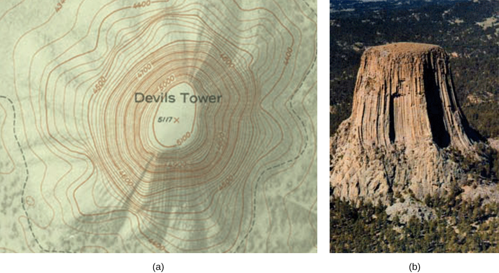
A topographical map along a ridge has roughly parallel elevation lines, similar to the equipotential lines in
[link] . (a) A topographical map of Devil’s Tower, Wyoming. Lines that are close together indicate very steep terrain. (b) A perspective photo of Devil’s Tower shows just how steep its sides are. Notice the top of the tower has the same shape as the center of the topographical map.
Calculating equipotential lines
You have seen the equipotential lines of a point charge in
[link] . How do we calculate them? For example, if we have a
charge at the origin, what are the equipotential surfaces at which the potential is (a) 100 V, (b) 50 V, (c) 20 V, and (d) 10 V?
Strategy
Set the equation for the potential of a point charge equal to a constant and solve for the remaining variable(s). Then calculate values as needed.
Solution
In
, let
V be a constant. The only remaining variable is
r ; hence,
. Thus, the equipotential surfaces are spheres about the origin. Their locations are:
;
;
;
.
Significance
This means that equipotential surfaces around a point charge are spheres of constant radius, as shown earlier, with well-defined locations.
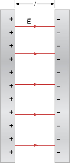
Potential difference between oppositely charged parallel plates
Two large conducting plates carry equal and opposite charges, with a surface charge density
of magnitude
as shown in
[link] . The separation between the plates is
. (a) What is the electric field between the plates? (b) What is the potential difference between the plates? (c) What is the distance between equipotential planes which differ by 100 V?
The electric field between oppositely charged parallel plates. A portion is released at the positive plate.
Strategy
(a) Since the plates are described as “large” and the distance between them is not, we will approximate each of them as an infinite plane, and apply the result from Gauss’s law in the previous chapter.
(b) Use
.
(c) Since the electric field is constant, find the ratio of 100 V to the total potential difference; then calculate this fraction of the distance.
Solution
The electric field is directed from the positive to the negative plate as shown in the figure, and its magnitude is given by
To find the potential difference
between the plates, we use a path from the negative to the positive plate that is directed against the field. The displacement vector
and the electric field
are antiparallel so
The potential difference between the positive plate and the negative plate is then
The total potential difference is 500 V, so 1/5 of the distance between the plates will be the distance between 100-V potential differences. The distance between the plates is 6.5 mm, so there will be 1.3 mm between 100-V potential differences.
Significance
You have now seen a numerical calculation of the locations of equipotentials between two charged parallel plates.