Lecture 1: introduction to signals

Lecture #1:

INTRODUCTION TO SIGNALS

Motivation: To describe signals, both man-made and naturally occurring, in forms of mathematical expressions in time and frequency domains.

Outline:

• Classification of signals

• Building-block signals — complex exponentials, impulses.

• Conclusions

Signals and systems

This subject deals with mathematical methods used to describe signals and to analyze and synthesize systems.

• Signals are variables that carry information
• Systems process input signals to produce output signals.

Today — SIGNALS; Next time — SYSTEMS.

Demonstration of different types of signals

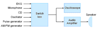
I. CLASSIFICATION OF SIGNALS

Identity of the independent variable

Time is often the independent variable for signals. For example, the electrical activity of the heart recorded with electrodes on the surface of the chest — the electrocardiogram (ECG or EKG).

Generic time

The term time is often used generically to represent the independent variable of a signal. The independent variable may be a spatial variable as in an image. Here color information is specified as a function of position.

Dimensionality of the independent variable

The independent variable can be 1-D (time t in the EKG signal) or 2-D (space x, y in the image), 3-D, or N-D.

In this course, we shall consider largely 1-D signals, but signals in many applications (e.g., radio astronomy, medical imaging, seismometry) have multiple dimensions.

1. Continuous time (CT) and discrete time (DT) signals

CT signals take on real or complex values as a function of an independent variable that ranges over the real numbers and are denoted as x(t). DT signals take on real or complex values as a function of an independent variable that ranges over the integers and are denoted as x[n]. Note the subtle use of parentheses and square brackets to distinguish between CT and DT signals.

For example, consider the image shown on the left and its DT representation shown on the right

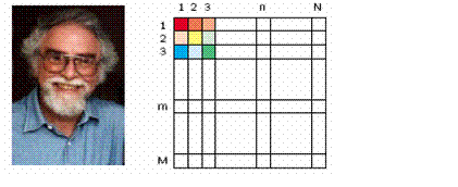
The image on the left consists of 302 × 435 picture elements (pixels) each of which is represented by a triplet of numbers {R,G,B} that encode the color. Thus, the signal is represented by c[n,m] where m and n are the independent variables that specify pixel location and c is a color vector specified by a triplet of hues {R,G,B} (red, green, and blue).

2/ Real and complex signals

Signals can be real, imaginary, or complex. An important class of signals are the complex exponentials:

• the CT signal x(t) = $e^{\text{st}}$ where is s is a complex number,
• the DT signal x[n] = $z^n$ where z is a complex number.

Q. Why do we deal with complex signals?

A. They are often analytically simpler to deal with than real signals.

For both exponential CT (x(t) = $e^{\text{st}}$ ) and DT (x[n] = $z^n$ ) signals, x is a complex quantity. To plot x, we can choose to plot either its magnitude and angle or its real and imaginary parts - whichever is more convenient for the analysis.

For example, suppose s = jπ/8