

| << Chapter < Page | Chapter >> Page > |
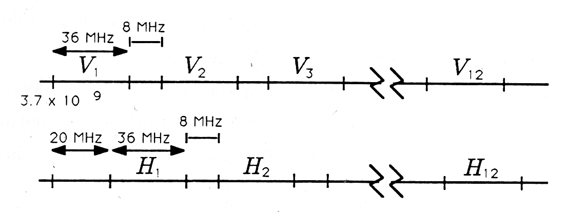
An Aside on Hertz and Seconds. The abbreviation Hz stands for hertz, or cycles/second. It is used to describe the frequency of a sinusoidal signal. For example, house current is 60 Hz, meaning that it has 60 cycles each second. The inverse of Hz is seconds or, more precisely, seconds/cycle, the period of 1 cycle. For example, the period of 1 cycle for house current is 1/60 second. When we are dealing with sound, electricity, and electromagnetic radiation, we need a concise language for dealing with signals and waves whose frequencies range from 0 Hz (called DC or direct current) to Hz (visible light). Table 1 summarizes the terms and symbols used to describe the frequency and period of signals that range in frequency from 0 Hz to Hz.
| Frequency | Period | |||||
|---|---|---|---|---|---|---|
| Hz | Term | Units | Seconds | Term | Units | Example |
| Hz | hertz | 1 Hz | sec | second | 1 sec | battery current: 0 Hz
house current: 60 Hz |
| kHz | kilohertz | 10 3 Hz | msec | millisecond | 10 -3 sec | midfrequency sound |
| MHz | megahertz | 10 6 Hz | µsec | microsecond | 10 -6 sec | clock frequencies in microcomputers |
| GHz | gigahertz | 10 9 Hz | nsec | nanosecond | 10 -9 sec | microwave radiation for satellite communication |
| THz | terahertz | 10 12 Hz | psec | picosecond | 10 -12 sec | infrared radiation |
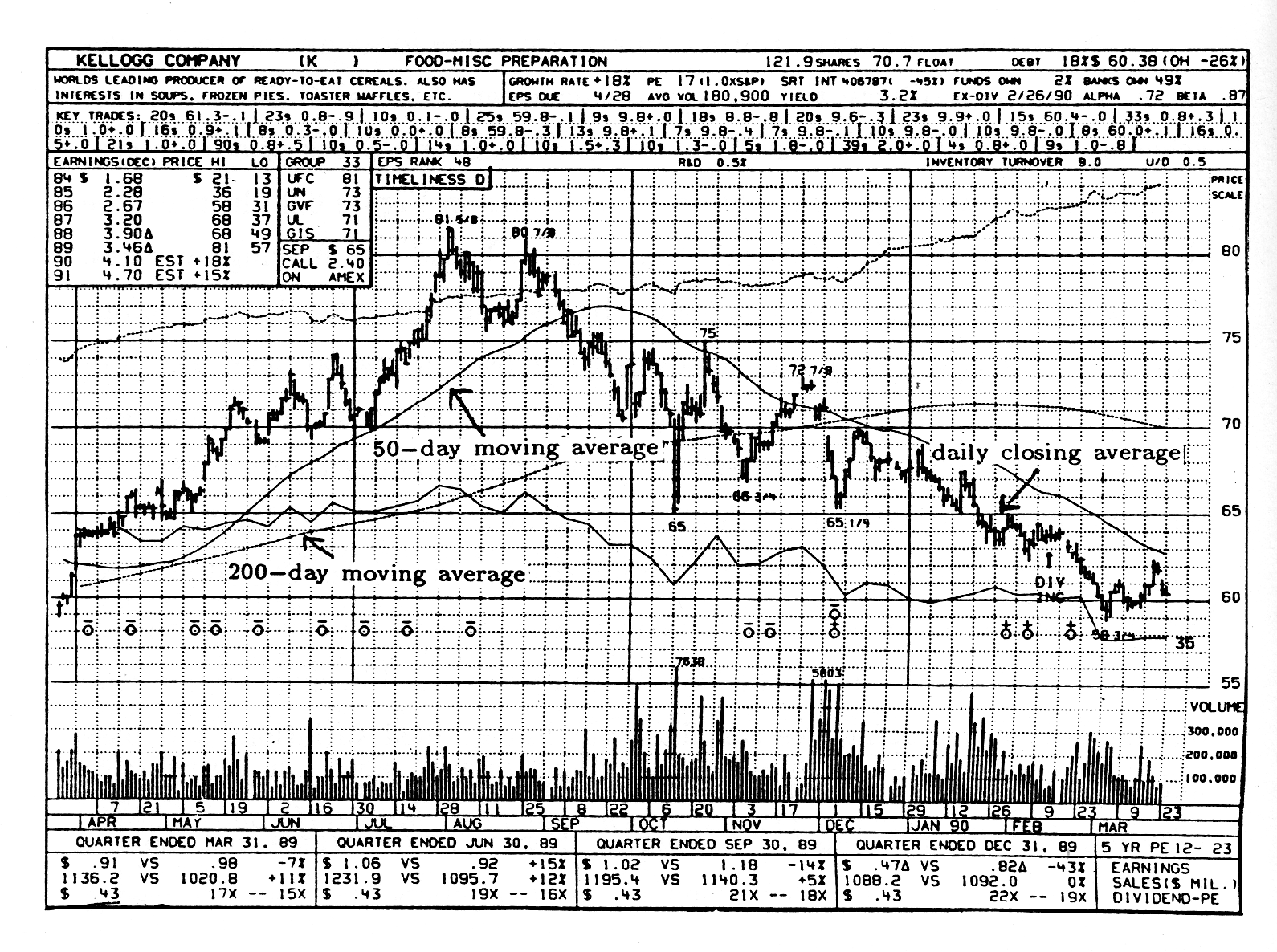
Numerical Filters. Rather amazingly, these ideas extend to the domain of numerical filters, the topic of this chapter. Numerical filters are just schemes for weighting and summing strings of numbers. Stock prices are typically averaged with numerical filters. The curves in Figure 2 illustrate the daily closing average for Kellogg's common stock and two moving averages. The 50-day moving average is obtained by passing the daily closing average through a numerical filter that averages the most current 50 days' worth of closing averages. The 200-day moving average for the stock price is obtained by passing the daily closing prices through a numerical filter that averages the most current 200 days' worth of daily closing averages. The daily closing averages show fine-grained variation but tend to conceal trends. The 50-day and 200-day averages show less fine-grained variation but give a clearer picture of trends. In fact, this is one of the key ideas in numerical filtering: by selecting our method of averaging, we can filter out fine-grained variations and pass long-term trends (or vice versa), or we can filter out periodic variations and pass nonperiodic variations (or vice versa). Figure 2 illustrates that moving averages typically lag increasing sequences of numbers and lead decreasing sequences. Can you explain why?
We will call any algorithm or procedure for transforming one set of numbers into another set of numbers a numerical filter or digital filter . Digital filters, consisting of memories and arithmetic logic units (ALUs), are implemented in VLSI circuits and used for communication, control, and instrumentation. They are also implemented in random–or semicustom–logic circuits and in programmable microcomputer systems. The inputs to a digital filter are typically electronic measurements that are produced by A/D (analog-to-digital) conversion of the output of an electrical or mechanical sensor. The outputs of the filter are “processed,” “filtered,” or “smoothed” versions of the measurements. In your more advanced courses in electrical and computer engineering you will study signal processing and system theory, assembly language programming, microprocessor system development, and computer design. In these courses you will study the design and programming of hardware that may be used for digital filtering.
Notification Switch
Would you like to follow the 'A first course in electrical and computer engineering' conversation and receive update notifications?

|
|

|
|

|
|

|
|
|
|
|

|
|
|
|
|

|
|

|
|
|
|