

| << Chapter < Page | Chapter >> Page > |
The logistic differential equation is an autonomous differential equation, so we can use separation of variables to find the general solution, as we just did in [link] .
Step 1: Setting the right-hand side equal to zero leads to and as constant solutions. The first solution indicates that when there are no organisms present, the population will never grow. The second solution indicates that when the population starts at the carrying capacity, it will never change.
Step 2: Rewrite the differential equation in the form
Then multiply both sides by and divide both sides by This leads to
Multiply both sides of the equation by and integrate:
The left-hand side of this equation can be integrated using partial fraction decomposition. We leave it to you to verify that
Then the equation becomes
Now exponentiate both sides of the equation to eliminate the natural logarithm:
We define so that the equation becomes
To solve this equation for first multiply both sides by and collect the terms containing on the left-hand side of the equation:
Next, factor from the left-hand side and divide both sides by the other factor:
The last step is to determine the value of The easiest way to do this is to substitute and in place of in [link] and solve for
Finally, substitute the expression for into [link] :
Now multiply the numerator and denominator of the right-hand side by and simplify:
We state this result as a theorem.
Consider the logistic differential equation subject to an initial population of with carrying capacity and growth rate The solution to the corresponding initial-value problem is given by
Now that we have the solution to the initial-value problem, we can choose values for and and study the solution curve. For example, in [link] we used the values and an initial population of deer. This leads to the solution
Dividing top and bottom by gives
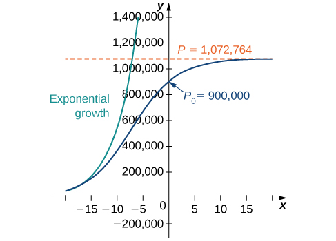
This is the same as the original solution. The graph of this solution is shown again in blue in [link] , superimposed over the graph of the exponential growth model with initial population and growth rate (appearing in green). The red dashed line represents the carrying capacity, and is a horizontal asymptote for the solution to the logistic equation.
Notification Switch
Would you like to follow the 'Calculus volume 2' conversation and receive update notifications?

|
|

|
|

|
|

|
|

|
|

|
|

|
|
|
|
|

|
|

|