Working under the assumption that the population grows according to the logistic differential equation, this graph predicts that approximately
years earlier
the growth of the population was very close to exponential. The net growth rate at that time would have been around
per year. As time goes on, the two graphs separate. This happens because the population increases, and the logistic differential equation states that the growth rate decreases as the population increases. At the time the population was measured
it was close to carrying capacity, and the population was starting to level off.
The solution to the logistic differential equation has a point of inflection. To find this point, set the second derivative equal to zero:
Setting the numerator equal to zero,
As long as
the entire quantity before and including
is nonzero, so we can divide it out:
Solving for
Notice that if
then this quantity is undefined, and the graph does not have a point of inflection. In the logistic graph, the point of inflection can be seen as the point where the graph changes from concave up to concave down. This is where the “leveling off” starts to occur, because the net growth rate becomes slower as the population starts to approach the carrying capacity.
A population of rabbits in a meadow is observed to be
rabbits at time
After a month, the rabbit population is observed to have increased by
Using an initial population of
and a growth rate of
with a carrying capacity of
rabbits,
Write the logistic differential equation and initial condition for this model.
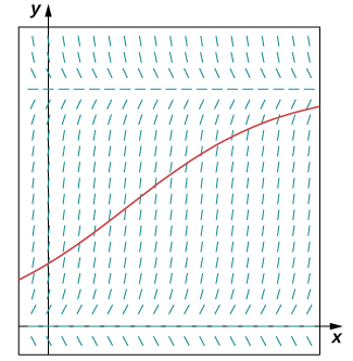
Draw a slope field for this logistic differential equation, and sketch the solution corresponding to an initial population of
rabbits.
Solve the initial-value problem for
Use the solution to predict the population after
year.
Student project: logistic equation with a threshold population
An improvement to the logistic model includes a
threshold population . The threshold population is defined to be the minimum population that is necessary for the species to survive. We use the variable
to represent the threshold population. A differential equation that incorporates both the threshold population
and carrying capacity
is
where
represents the growth rate, as before.
The threshold population is useful to biologists and can be utilized to determine whether a given species should be placed on the endangered list. A group of Australian researchers say they have determined the threshold population for any species to survive:
adults. (Catherine Clabby, “A Magic Number,”
American Scientist 98(1): 24, doi:10.1511/2010.82.24. accessed April 9, 2015, http://www.americanscientist.org/issues/pub/a-magic-number). Therefore we use
as the threshold population in this project. Suppose that the environmental carrying capacity in Montana for elk is
Set up
[link] using the carrying capacity of
and threshold population of
Assume an annual net growth rate of
Draw the direction field for the differential equation from step
along with several solutions for different initial populations. What are the constant solutions of the differential equation? What do these solutions correspond to in the original population model (i.e., in a biological context)?
What is the limiting population for each initial population you chose in step
(Hint: use the slope field to see what happens for various initial populations, i.e., look for the horizontal asymptotes of your solutions.)
This equation can be solved using the method of separation of variables. However, it is very difficult to get the solution as an explicit function of
Using an initial population of
elk, solve the initial-value problem and express the solution as an implicit function of
or solve the general initial-value problem, finding a solution in terms of