2.1 Analysis of time series

Analysis of time-series

Introduction

This module offers a brief introduction of some of the issues that arise in the analysis of time-series. Most of the topics covered are those that we attacked first by statisticians and economists. As such they do not demand the more sophisticated tools used by the more modern approaches to time-series. In spite of these shortcomings, they should give you some understanding of the issues that arise with the use of times-series in econometric analyses. One final note of explanation is necessary. These notes are designed to give you a brief introduction to how Stata handles time-series data. These notes are not a substitute for reading the Stata manual, completing a forecasting course, or reading standard texts on the rather complicated field.

Time-series analysis in Stata

Throughout this module we work with US macroeconomic data included in the MS Excel file Macro data.xls . The variables are real level of investments (RINV), real gross national product (RGNP), and real interest rate (RINTRATE). The real interest rate is approximated by the difference between the nominal interest rate and the rate of change of the price index from the previous year. The data are for the years 1963 to 1982. You can replicate the analysis done here by copying this data set into a Stata file.

The first step after entering the data set into Stata , is to declare that the data set is a time-series. The command to do this is:

. tsset year

The data set can be broken into any number of time periods including daily, weekly, monthly, quarterly, halfyearly, yearly and generic. See StataCorp [2003:119-130] for more detail on this command.

Assume that we want to estimate the following regression:

using the data set in the appendix. Figure 1 shows this regression command and the resultant output.

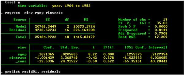
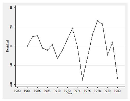
On the surface the estimates seem “reasonable” because the signs on the two explanatory variables are what theory predicts they should be and the parameter for real GNP is statistically different from zero. However, an examination of the residuals shown in Figure 2 suggest that the error terms might exhibit autocorrelation.

There are several issues that arise here. First, what sort of models can we use to account for autocorrelation? Second, what sorts of tests exist for detecting the existence of autocorrelation? We begin with the first of these questions by introducing the concept of first-order autocorrelation. Consider the following model:

We say that this model exhibits first-order autocorrelation if the error terms can be written as:

where ${\mu }_t~N\left(0,{\sigma }^2\right).$ Equation (3) implies that the error terms in (2) are correlated with each other. It is rather easy to show that, while the estimates of the unknown parameters are unbiased, the estimates of the standard errors are biased—downward if $1>\rho >0$ and upward if $-1<\rho <0.$ This conclusion holds as long as the source of the autocorrelation is due to (3). If, on the other hand, the source of autocorrelation among the error terms in (2) is due to omitted explanatory variables (whose effects are absorbed in the error term), we have a potentially more serious problem. In particular, if the omitted explanatory variables are correlated with the included explanatory variables (as is often true in time-series), then the estimates of the unknown slope parameters are also biased.