2.1 Analysis of time series  (Page 2/6)

For the moment we will assume that Equations (2) and (3) are true representations of the world. What then can we do to estimate (2)? What we need to do is find a way to transform (2) so that the error term of whatever regression we estimate does not exhibit autocorrelation. In time period $t-1$ we have:

Multiply (4) by $\rho$ to get:

Now subtracting (5) from (4) gives:

$$y_t-\rho y_{t-1}={\beta }_0+{\beta }_1{x}_t+{\epsilon }_t-\left(\rho {\beta }_0+\rho {\beta }_1{x}_{t-1}+\rho {\epsilon }_{t-1}\right)$$

or, equivalently,

$$\left(y_t-\rho y_{t-1}\right)={\beta }_0\left(1-\rho \right)+{\beta }_1\left(x_t-\rho x_{t-1}\right)+\left({\epsilon }_t-\rho {\epsilon }_{t-1}\right).$$

Let

$$y_t^{\ast }=y_{t-1}-\rho y_{t-1},$$

$${\beta }_0^{\ast }={\beta }_0\left(1-\rho \right),$$

and

$$x_t^{\ast }=x_{t-1}-\rho x_{t-1}.$$

Remember that (3) implies that ${\mu }_t={\epsilon }_t-\rho {\epsilon }_{t-1}.$ Thus, we have:

where ${\mu }_t~N\left(0,{\sigma }^2\right).$ Thus, we have a regression for which the OLS estimates will be BLUE (Best Linear Unbiased Estimator) if we only knew the true value of $\rho .$

Cochran and Orcutt [1949] use this algebra to suggest one way to estimate (6). The estimation entails several steps. First, you use OLS to estimate (2). Second, you estimate (3) using the residuals from the first stage to approximate ${\epsilon }_t.$ This regression gives an estimate of $\rho .$ In the third step, you use the estimate of $\rho$ to construct estimates of $y_t^{\ast }$ and $x_t^{\ast }.$ In the fourth step, you use the estimates of $y_t^{\ast }$ and $x_t^{\ast }$ to estimate (6); this will yield new estimates of ${\beta }_0$ and ${\beta }_1$ . You then repeat step (2) using these new estimates of ${\beta }_0$ and ${\beta }_1$ to calculate the residuals and then repeat with steps (3) and (4). You continue the process until the estimate of $\rho$ does not change anymore (i.e., until the change in the estimate of $\rho$ is less than some value chosen by the researcher). There are a multitude of alternative ways of estimating $\rho .$ [See Greene (1990): Chapter 15 for a full discussion of these methods.] Once you have an estimator for $\rho ,$ there exist two major ways of completing the estimation—the Cochran-Orcutt procedure described above and the Prais-Winsten (1954) estimator. The latter estimation procedure does not involve dropping the first observation (as does the Cochran-Orcutt) estimator. In large samples these two estimation techniques are likely to be very similar. In small samples the two techniques may produce estimates that are substantially different.

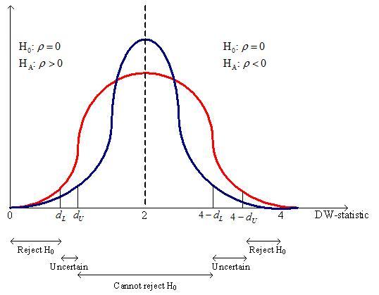
We now turn to the issue of detecting the existence of autocorrelation. In what follows we focus mainly on the detection of first-order autocorrelation as shown in Equation (3). We can use the Durbin-Watson test to see if our suspicions are correct. The Durbin-Watson statistic tests the hypothesis:

The details of the test statistic can be found in any econometrics textbook and need not detain us here. What you need to know about the DW-statistic are (1) it has a mean value of 2; (2) because its distribution lies between two limiting distributions, we need to look at two critical values. For this reason there are two critical values—one for each of the limiting distributions. Figure 3 illustrates the probability distribution function (pdf) for the Durbin-Watson statistic. The true pdf lies somewhere between the blue pdf and the red pdf. What is shown in the figure is the point below which, say, 5 percent of the distribution lies for each distribution. The true critical point lies somewhere between $d_L$ and $d_U$ These values are relevant to testing the null hypothesis of no autocorrelation against the alternative hypothesis of positive autocorrelation $(\text{i}\text{. e}\text{.,}$ $\rho >0).$