<< Chapter < Page Chapter >> Page >

These are determined from N initial conditions which must be specified. These conditions result in a set of N algebraic equations that need to be solved to obtain the initial conditions. We shall find another, and simpler, method to determine these coefficients later.

2/ Steady-state

Assume the particular solution is not zero. Then the particular solution dominates after some time, if the homogeneous solution decays more rapidly than does the particular solution. When this occurs, we call the resulting particular solution the steady-state response. Steady-state occurs if each term in the homogeneous solution decays more rapidly than the particular solution. Thus, steady-state occurs if

lim t e λ n t e st 0 for all λ n size 12{ {"lim"} cSub { size 8{t rightarrow infinity } } lline { {e rSup { size 8{λ rSub { size 6{n} } t} } } over {e rSup { ital "st"} } } rline size 12{ rightarrow 0`` ital "for"`` ital "all"``λ rSub {n} }} {}

Thus

lim t e ( λ n s ) t 0 for all λ n size 12{ {"lim"} cSub { size 8{t rightarrow infinity } } lline e rSup { size 8{ \( λ rSub { size 6{n} } - s \) t} } rline rightarrow 0`` ital "for"`` ital "all"``λ rSub {n} } {}

which implies that

R { λ n s } 0 for all λ n size 12{R lbrace λ rSub { size 8{n} } - s rbrace 0`` ital "for"`` ital "all"``λ rSub { size 8{n} } } {}

Thus, steady-state occurs when

R { λ n } < R { s } size 12{R lbrace λ rSub { size 8{n} } rbrace<R lbrace s rbrace } {} for all λ n size 12{λ rSub { size 8{n} } } {}

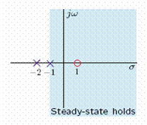
provided the particular solution is not zero. The conditions for steady state are depicted in the complex s plane below.

The particular solution dominates for s in the shaded region, and the total solution equals the steady-state solution i.e.,

y ( t ) = XH ( s ) e st size 12{y \( t \) = ital "XH" \( s \) e rSup { size 8{ ital "st"} } } {}

For which conditions is the particular solution zero? Suppose

H ( s ) = s 1 ( s + 1 ) ( s + 2 ) size 12{H \( s \) = { {s - 1} over { \( s+1 \) \( s+2 \) } } } {}

The particular solution dominates for s in the shaded region, and the total solution equals the steady-state solution except when s = 1 because at this value i.e.,

y ( t ) = XH ( 1 ) e s = 0 size 12{y \( t \) = ital "XH" \( 1 \) e rSup { size 8{s} } =0} {}

so that the particular solution is zero and steady -state does not occur.

IX. LINEAR DIFFERENCE EQUATIONS ARISE IN MANY DIFFERENT CONTEXTS

1/ Electric ladder network

r is the series resistance and g is the shunt conductance.

KCL at the central node yields

v o [ n 1 ] v o [ n ] r + v o [ n + 1 ] v o [ n ] r + g ( v i [ n ] v o [ n ] = 0 size 12{ { {v rSub { size 8{o} } \[ n - 1 \] - v rSub { size 8{o} } \[ n \]} over {r} } + { {v rSub { size 8{o} } \[ n+1 \] - v rSub { size 8{o} } \[ n \]} over {r} } +g \( v rSub { size 8{i} } \[ n \] - v rSub { size 8{o} } \[ n \]=0} {}

which yields the linear difference equation

v o [ n + 1 ] + ( 2 + rg ) v o [ n ] v o [ n 1 ] = rgv i [ n ] size 12{ - v rSub { size 8{o} } \[ n+1 \] + \( 2+ ital "rg" \) v rSub { size 8{o} } \[ n \]- v rSub { size 8{o} } \[ n - 1 \] = ital "rgv" rSub { size 8{i} } \[ n \]} {}

2/ Interest and accumulation

Let us consider a simple model of the accumulation of wealth through savings. At the end of year n you deposit x[n] dollars in the bank which pays an annual interest of r. Your accumulation at the end of year n is y[n]dollars. Therefore,

y [ n + 1 ] = y [ n ] + ry [ n ] + x [ n ] size 12{y \[ n+1 \] =y \[ n \]+ ital "ry" \[ n \] +x \[ n \]} {}

We can rewrite this equation as

y[n+1] − (1+r)y[n]= x[n]

This difference equation can be realized in a block diagram as shown below.

D is a unit delay unit.

3/ Discretized CT system

An important application of DT systems is a numerical simulation of a CT system. For example, consider the CT lowpass filter shown below.

The differential equation is

dv o ( t ) dt = 1 RC v o ( t ) + 1 RC v i ( t ) size 12{ { { ital "dv" rSub { size 8{o} } \( t \) } over { ital "dt"} } = - { {1} over { ital "RC"} } v rSub { size 8{o} } \( t \) + { {1} over { ital "RC"} } v rSub { size 8{i} } \( t \) } {}

To solve this equation numerically in a computer, the CT signals are discretized and the derivative is approximated.

To discretize the signals, we can define DT signals as samples of CT signals, i.e.,

v i [ n ] = v i ( t ) t = nT = v i ( nT ) size 12{v rSub { size 8{i} } \[ n \] =v rSub { size 8{i} } \( t \) \lline rSub { size 8{t= ital "nT"} } =v rSub { size 8{i} } \( ital "nT" \) } {} and v o [ n ] = v o ( t ) t = nT = v o ( nT ) size 12{v rSub { size 8{o} } \[ n \] =v rSub { size 8{o} } \( t \) \lline rSub { size 8{t= ital "nT"} } =v rSub { size 8{o} } \( ital "nT" \) } {}

The derivative can be approximated as follows

dv o ( t ) dt t = nT v o ( ( n + 1 ) T ) = v o ( nT ) T size 12{ { { ital "dv" rSub { size 8{o} } \( t \) } over { ital "dt"} } \lline rSub { size 8{t= ital "nT"} } approx { {v rSub { size 8{o} } \( \( n+1 \) T \) =v rSub { size 8{o} } \( ital "nT" \) } over {T} } } {}

Therefore, we can approximate the differential equation as

v o ( ( n + 1 ) T ) = v o ( nT ) T = 1 RC v o ( nT ) + 1 RC v i ( nT ) size 12{ { {v rSub { size 8{o} } \( \( n+1 \) T \) =v rSub { size 8{o} } \( ital "nT" \) } over {T} } = - { {1} over { ital "RC"} } v rSub { size 8{o} } \( ital "nT" \) + { {1} over { ital "RC"} } v rSub { size 8{i} } \( ital "nT" \) } {}

which can be written as

v o [ n + 1 ] = ( 1 T RC ) v o [ n ] + ( T RC ) v i [ n ] size 12{v rSub { size 8{o} } \[ n+1 \] = \( 1 - { {T} over { ital "RC"} } \) v rSub { size 8{o} } \[ n \]+ \( { {T} over { ital "RC"} } \) v rSub { size 8{i} } \[ n \] } {}

Let α size 12{α} {} = T/(RC). Then the difference equation is

v o [ n + 1 ] = ( 1 α ) v o [ n ] + αv i [ n ] size 12{v rSub { size 8{o} } \[ n+1 \] = \( 1 - α \) v rSub { size 8{o} } \[ n \]+αv rSub { size 8{i} } \[ n \] } {}

This equation can be solved iteratively for a given input and initial condition. Assume that v i [ n ] = u [ n ] size 12{v rSub { size 8{i} } \[ n \] =u \[ n \]} {} and that v o [ 0 ] = 0 size 12{v rSub { size 8{o} } \[ 0 \] =0} {} then

Get Jobilize Job Search Mobile App in your pocket Now!

Get it on Google Play Download on the App Store Now


Source:  OpenStax, Signals and systems. OpenStax CNX. Jul 29, 2009 Download for free at http://cnx.org/content/col10803/1.1
Google Play and the Google Play logo are trademarks of Google Inc.

Notification Switch

Would you like to follow the 'Signals and systems' conversation and receive update notifications?

Ask