

| << Chapter < Page | Chapter >> Page > |
Now we wish to find the coefficients of . If we multiply by and integrate, we get:
Then equating the first and last lines, we have a formula for recovering :
This derivation is valid for as large of as we want. In fact, the most general application of this is infinite series of sine waves.
Additionally, we can do the same thing with sums of cosines. If , then we can recover the coefficients in the same way (Exercise 3.1):
And if we have a function that is a mix of the two, such as
we can extract the coefficients by the same equations as above (Exercise 3.2).
Now we see why the trapezoid rule was so important. In order to recover the sine coefficients of a function, we need to be able to find the integral of
multiplied against different sine functions. We can do this pretty well with our trapezoid code. To show this method in action, we show the code
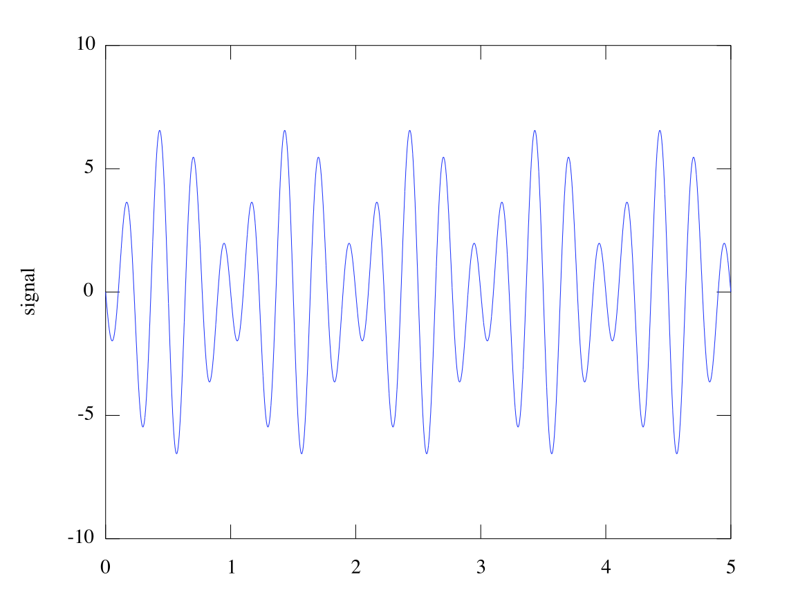
myfreq.m (full code in Appendix). We'll walk through it here. First, we create a sum of sine waves:
T = 5;% duration of signal
dt = 0.001;     % time between signal samplest = 0:dt:T;
N = length(t);y = 2.5*sin(3*2*pi*t) - 4.2*sin(4*2*pi*t);    % a 2-piece wave
plot(t,y)xlabel('time   (seconds)')
ylabel('signal')for f = 1:5,     % compute the amplitudes as ratios of areas
    a(f) = trapz(t,y.*sin(f*2*pi*t))/trapz(t,sin(f*2*pi*t).^2);end
Let's break down the syntax of this operation. We loop through the computation five times, each time representing a frequency
j from 1 to 5. Within the loop, the first
mytrapz is the integral we care about. We give it two arguments:
t and
y.*sin(j*2*pi*t) . The first, “
t ", is simply the time grid that we will approximately integrate over. The second corresponds to
, as in equation
[link] . Note that
j is the frequency we are testing. The operator (
.* ) performs
elementwise multiplication, that is, multiplying the corresponding elements in each array. (Many operators such as
+ and
sin() automatically do this.) Thus each entry in the
y.*sin(j*2*pi*t) corresponds to one in
t .
The second instance of
mytrapz() is just normalization (accounts for the length of the wave). After this, we plot the recovered coefficients against the originals. This effectively checks the error in our process.
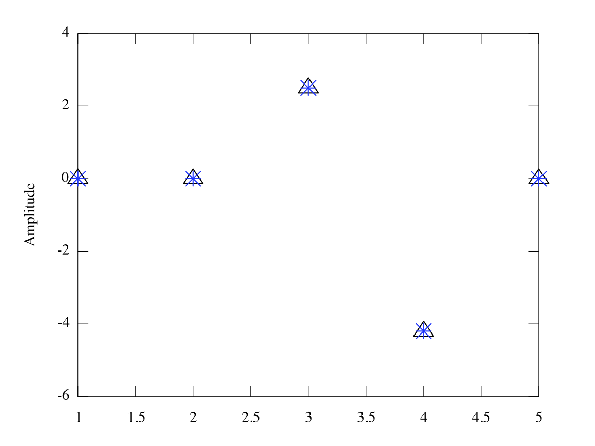
figure
plot(1:5,a,'ko')    % plot the amplitudes vs frequencyhold on
plot(1:5, [0 0 2.5 -4.2 0], 'b*')
As we can see from [link] , our method works well.
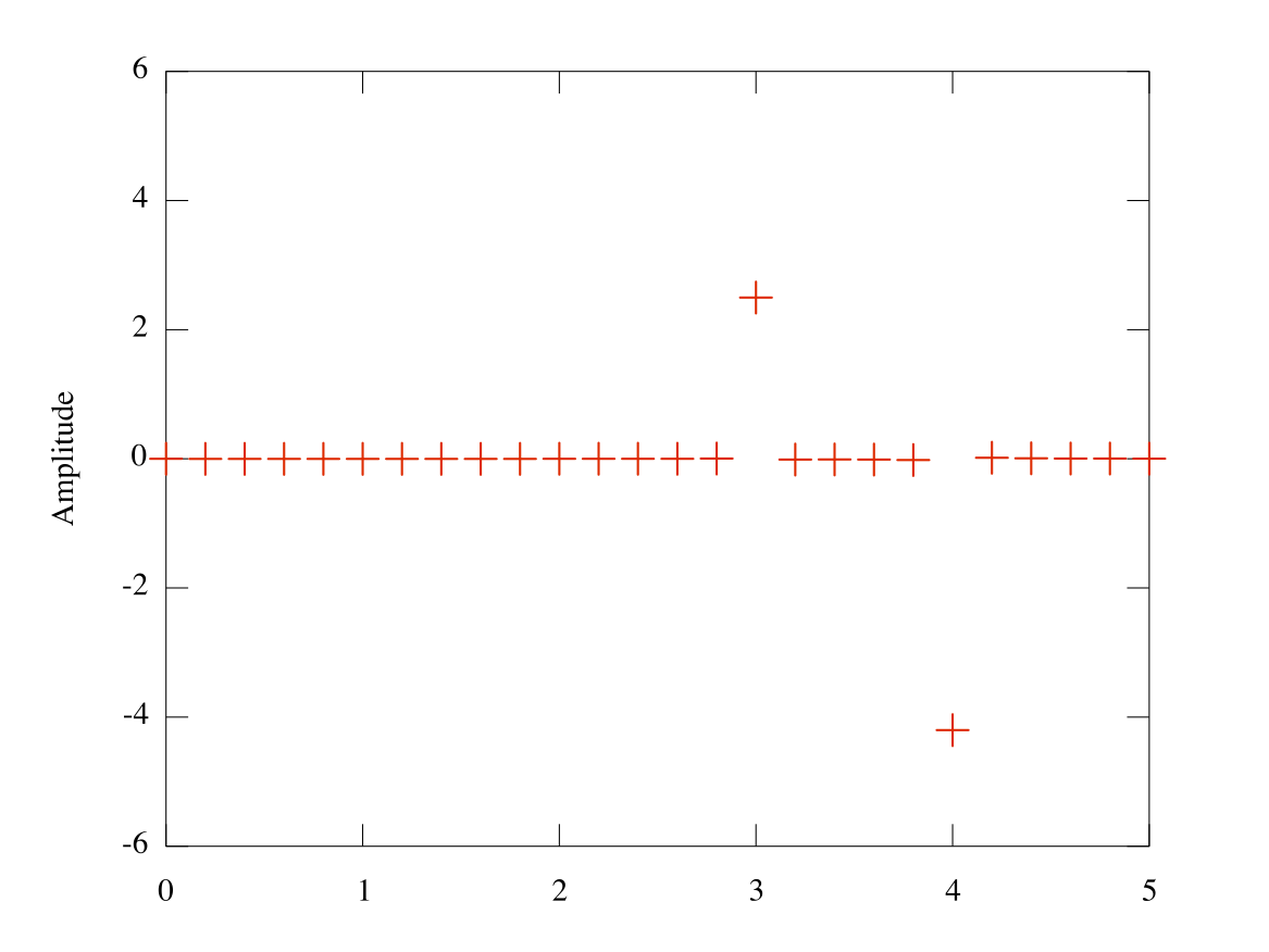
The remainder of the code uses the Matlab function
fft() . This stands for “Fast Fourier Transform." This transforms maps a function from the
time domain (the way we normally think about it) to the
frequency domain. Basically, we express a signal in terms of the frequency coefficients of which it is composed. The plots from this analysis confirm that our analysis is the same as that of the Matlab-tested functions.
Notification Switch
Would you like to follow the 'The art of the pfug' conversation and receive update notifications?

|
|

|
|

|
|

|
|

|
|

|
|

|
|

|
|

|
|

|