

| << Chapter < Page | Chapter >> Page > |
You may be pleasantly surprised to hear that
any periodic function can be broken down into an infinite sum of sine and cosine waves. The elements of such a sum are together called a Fourier Series. The method for recovering the coefficients of the Fourier Series for any periodic function are the same as in equation
[link] . Thus we create a function that will find the decomposition of any function. We do this in
myfourier.m . The entire code is in the appendix, but it uses very similar ideas as in
myfreq() (above).
function [freq mag] = myfourier(y, sr, use_fft, plot_on)(...some code skipped...)

for n = 1 : numel(freq)    %obtain coefficient for freqency nth frequency [freq(n)]
    sinmag(n) = mytrapz(t, y.*sin(freq(n)*2*pi*t), 1);    cosmag(n) = mytrapz(t, y.*cos(freq(n)*2*pi*t), 1);
end
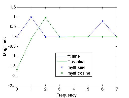
As a test, we compare the “answer"
fft code with our own for an arbitrary function and find good agreement:
3.1 Suppose . Then prove Equation [link] that helps recover the coefficients:
3.2 Suppose is an infinite sum of sine and cosine waves:
Show that Equations [link] and [link] , which give expressions for and , are still valid.
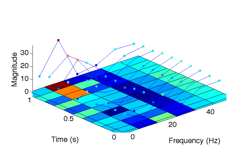
Here is the application we have been seeking the whole time. Given an EEG signal, we would like to find its corresponding Fourier series. We have just built up the tools to decompose the signal into component frequencies. This is useful, but the brain changes over time, and we want to be able to track changes in the signal over time. One way to do this is the spectrogram, or the short-term Fourier transform. It allows us to watch the way a signal changes over time.
The idea behind the Short-time Fourier Transform is that we break up the signal into several time windows, then take the Fourier transform of each one of these. In Figure 10, we analyze the function from time to . First, we break it up into 10 segments of 100 ms each. Each segment corresponds to one block in the “Time" dimension. The line in that block is the amplitudes of sine and cosine waves from the Fourier transform of the function over that time window. The colors on the plane below it represent the amplitude of that frequency in that time interval. The higher the amplitude, the closer to red, and the lower, the closer to blue. The resulting image that we get is called a spectrogram .
To code something like this, we consider each time window separately. This takes the form of a loop:
function [stft_plot freq tm] = my_stft(y, dt, win_len)(...some code skipped...)
for n = 1:Nwindow    %isolate the part of the signal we want to deal with
    sig_win = y((n-1)*win_len + 1 : n*win_len);
Within this window, we perform the Fourier Transform (using our homemade code!) and record it:
    %perform the fourier transform
    [mg freq] = myfourier(sig_win, dt, 1);
    sm(:,n) = mg(:,1);
    cm(:,n) = mg(:,2);end
Notification Switch
Would you like to follow the 'The art of the pfug' conversation and receive update notifications?

|
|

|
|

|
|

|
|

|
|

|
|

|
|
|
|
|
|
|
|

|