<< Chapter < Page Chapter >> Page >

dx 2 t dt size 12{ { { ital "dx" rSub { size 8{2} } left (t right )} over { ital "dt"} } } {} = K M x 1 t size 12{ - { {K} over {M} } x rSub { size 8{1} } left (t right )} {} - B M x 2 t size 12{ { {B} over {M} } x rSub { size 8{2} } left (t right )} {} + 1 M f t size 12{ { {1} over {M} } f left (t right )} {} (5.46)

Để hệ thống cơ trên đây tương đương với mạch RLC nối tiếp của mạch điện.

Với sự tương đương giữa một hệ thống cơ và một hệ thống điện, việc thành lập trực tiếp các phương trình trạng thái cho một hệ thống cơ sẽ trở nên đơn giản.

Nếu ta xem khối lượng thì tương đương với điện cảm, hằng số lò xo K thì tương đương với nghịch đảo của điện dung 1/C .

Vậy có thể chỉ định v(t): vận tốc và fk(t): lực tác động lên lò xo như là các biến số trạng thái. Lý do là cái trước tương tự dòng điện trong cuộn cảm, và cái sau tương tự như điện thế ngang qua tụ.

Do đó phương trình trạng thái của hệ được viết bằng:

Lực trên khối lượng:

M dv ( t ) dt = Bv ( t ) f k ( t ) + f ( t ) size 12{M { { ital "dv" \( t \) } over { ital "dt"} } = - ital "Bv" \( t \) - f rSub { size 8{k} } \( t \) +f \( t \) } {} (5.47)

Vận tốc của lò xo :

1 k df k ( t ) dt = v ( t ) size 12{ { {1} over {k} } { { ital "df" rSub { size 8{k} } \( t \) } over { ital "dt"} } =v \( t \) } {} (5.48)

Phương trình trên thì giống như cách viết phương trình điện thế ngang qua 1 cuộn cảm. Còn phương trình dưới giống như phương trình ngang qua tụ.

Thí dụ đơn giản trên cho thấy các phương trình trạng thái và biến số trạng thái của 1 hệ thống động thì không duy nhất.

Thí dụ 5.3:

Xem 1 hệ thống như hình H.5_17a. Vì lò xo bị biến dạng khi chịu tác dụng của lực f(t) hai độ dời y1 và y2 phải được chỉ định cho 2 đầu mút của lò xo. Sơ đồ vật thể tự do của hệ vẽ ở hình H.5_17b.

Từ H.5_17b, các phương trình lực được viết :

f(t)=K[y1(t)-y2(t)] (5.49)

K [ y 1 ( t ) y 2 ( t ) ] = M d 2 y 2 ( t ) dt 2 + B dy 2 ( t ) dt size 12{K \[ y rSub { size 8{1} } \( t \) - y rSub { size 8{2} } \( t \) \] =M { {d rSup { size 8{2} } y rSub { size 8{2} } \( t \) } over { ital "dt" rSup { size 8{2} } } } +B { { ital "dy" rSub { size 8{2} } \( t \) } over { ital "dt"} } } {} (5.50)

Để viết các phương trình trạng thái của hệ thống, ta đặt:

X1(t)=y2(t)

X2(t)= dy 2 ( t ) dt size 12{ { { ital "dy" rSub { size 8{2} } \( t \) } over { ital "dt"} } } {}

Thì các phương trình (5.49) và (5.50) được viết lại:

dx 1 ( t ) dt = x 2 ( t ) size 12{ { { ital "dx" rSub { size 8{1} } \( t \) } over { ital "dt"} } =x rSub { size 8{2} } \( t \) } {} (5.51)

dx 2 ( t ) dt = B M x 2 ( t ) + 1 M f ( t ) size 12{ { { ital "dx" rSub { size 8{2} } \( t \) } over { ital "dt"} } = - { {B} over {M} } x rSub { size 8{2} } \( t \) + { {1} over {M} } f \( t \) } {} (5.52)

Nếu ta chỉ định vận tốc v(t) của khối lượng M là 1 trạng thái biến số , lực fk(t) trên lò xo là 1 biến số, thì:

dv ( t ) dt = B M v ( t ) + 1 M f k ( t ) size 12{ { { ital "dv" \( t \) } over { ital "dt"} } = - { {B} over {M} } v \( t \) + { {1} over {M} } f rSub { size 8{k} } \( t \) } {} (5.53)

fk(t)=f(t) (5.54)

Mạch điện tương đương với hệ cơ trên được vẽ ở hình H.5­_18.

Nếu muốn tìm độ dời y1(t) tại điển mà y(t) áp dụng vào, ta dùng hệ thức:

y 2 = f k ( t ) k + y 2 ( t ) = f ( t ) k + 0 t v ( τ ) + y 2 ( 0 ) size 12{y rSub { size 8{2} } = { {f rSub { size 8{k} } \( t \) } over {k} } +y rSub { size 8{2} } \( t \) = { {f \( t \) } over {k} } + Int rSub { size 8{0} } rSup { size 8{t} } {v \( τ \) dτ+y rSub { size 8{2} } \( 0 \) } } {} (5.55)

Trong đó y2(0) là độ dời ban đầu của khối lượng M .

Mặt khác, có thể giải cho y2(t) từ 2 phương trình trạng thái (5.51) và (5.52) và y1(t) được xác định bằng (5.49).

Thí dụ 5.4:

Hệ thống quay vẽ ở hình H.5_19 gồm 1 đầu thì cố định. Moment quán tính của dĩa quanh trục là J. Rìa của dĩa được lướt trên mặt phẳng và hệ số ma sát trượt là B. Bỏ qua quán tính của trục. Hằng số xoắn là K.

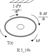
Giả sử 1 moment áp dụng vào hệ thống như hình vẽ:

Phương trình momen quanh trục được viết từ hình H.5_19b

T(t)= J d 2 θ ( t ) dt 2 + B ( t ) dt + ( t ) size 12{J { {d rSup { size 8{2} } θ \( t \) } over { ital "dt" rSup { size 8{2} } } } +B { {dθ \( t \) } over { ital "dt"} } +Kθ \( t \) } {} (5.62)

Hệ thống này tương tự như hệ thống chuyển động tịnh tiến ở H.5_16. Các phương trình trạng thái có thể viết bằng các định nghĩa các biến. x1(t)= θ ( t ) size 12{θ \( t \) } {}

dx 1 ( t ) dt = x 2 ( t ) size 12{ { { ital "dx" rSub { size 8{1} } \( t \) } over { ital "dt"} } =x rSub { size 8{2} } \( t \) } {}

Ngươì đọc có thể thực hiện các bước tiếp theo để viết phương trình trạng thái như là 1 bài tập.

Mô hình hóa động cơ dc.

Sơ lược về các lọai động cơ dc:

Motor DC có thể được xếp thành 2 loại : loại có từ thông thay đổi được và loại không có từ thông thay đổi được.

-Trong loại thứ nhất: Từ trường được tạo bởi cuộn cảm. Mà cuộn cảm thì đấu với 1 từ trường ngoài. Loại động cơ này lại được có thể chia làm 2 loại: kích từ nối tiếp và kích từ riêng.

H.5_19a, ký hiệu của động cơ DC kích từ nối tiếp. Cuộn cảm đấu nối tiếp với phần ứng.

Questions & Answers

differentiate between demand and supply giving examples
Lambiv Reply
differentiated between demand and supply using examples
Lambiv
what is labour ?
Lambiv
how will I do?
Venny Reply
how is the graph works?I don't fully understand
Rezat Reply
information
Eliyee
devaluation
Eliyee
t
WARKISA
hi guys good evening to all
Lambiv
multiple choice question
Aster Reply
appreciation
Eliyee
explain perfect market
Lindiwe Reply
In economics, a perfect market refers to a theoretical construct where all participants have perfect information, goods are homogenous, there are no barriers to entry or exit, and prices are determined solely by supply and demand. It's an idealized model used for analysis,
Ezea
What is ceteris paribus?
Shukri Reply
other things being equal
AI-Robot
When MP₁ becomes negative, TP start to decline. Extuples Suppose that the short-run production function of certain cut-flower firm is given by: Q=4KL-0.6K2 - 0.112 • Where is quantity of cut flower produced, I is labour input and K is fixed capital input (K-5). Determine the average product of lab
Kelo
Extuples Suppose that the short-run production function of certain cut-flower firm is given by: Q=4KL-0.6K2 - 0.112 • Where is quantity of cut flower produced, I is labour input and K is fixed capital input (K-5). Determine the average product of labour (APL) and marginal product of labour (MPL)
Kelo
yes,thank you
Shukri
Can I ask you other question?
Shukri
what is monopoly mean?
Habtamu Reply
What is different between quantity demand and demand?
Shukri Reply
Quantity demanded refers to the specific amount of a good or service that consumers are willing and able to purchase at a give price and within a specific time period. Demand, on the other hand, is a broader concept that encompasses the entire relationship between price and quantity demanded
Ezea
ok
Shukri
how do you save a country economic situation when it's falling apart
Lilia Reply
what is the difference between economic growth and development
Fiker Reply
Economic growth as an increase in the production and consumption of goods and services within an economy.but Economic development as a broader concept that encompasses not only economic growth but also social & human well being.
Shukri
production function means
Jabir
What do you think is more important to focus on when considering inequality ?
Abdisa Reply
any question about economics?
Awais Reply
sir...I just want to ask one question... Define the term contract curve? if you are free please help me to find this answer 🙏
Asui
it is a curve that we get after connecting the pareto optimal combinations of two consumers after their mutually beneficial trade offs
Awais
thank you so much 👍 sir
Asui
In economics, the contract curve refers to the set of points in an Edgeworth box diagram where both parties involved in a trade cannot be made better off without making one of them worse off. It represents the Pareto efficient allocations of goods between two individuals or entities, where neither p
Cornelius
In economics, the contract curve refers to the set of points in an Edgeworth box diagram where both parties involved in a trade cannot be made better off without making one of them worse off. It represents the Pareto efficient allocations of goods between two individuals or entities,
Cornelius
Suppose a consumer consuming two commodities X and Y has The following utility function u=X0.4 Y0.6. If the price of the X and Y are 2 and 3 respectively and income Constraint is birr 50. A,Calculate quantities of x and y which maximize utility. B,Calculate value of Lagrange multiplier. C,Calculate quantities of X and Y consumed with a given price. D,alculate optimum level of output .
Feyisa Reply
Answer
Feyisa
c
Jabir
the market for lemon has 10 potential consumers, each having an individual demand curve p=101-10Qi, where p is price in dollar's per cup and Qi is the number of cups demanded per week by the i th consumer.Find the market demand curve using algebra. Draw an individual demand curve and the market dema
Gsbwnw Reply
suppose the production function is given by ( L, K)=L¼K¾.assuming capital is fixed find APL and MPL. consider the following short run production function:Q=6L²-0.4L³ a) find the value of L that maximizes output b)find the value of L that maximizes marginal product
Abdureman
types of unemployment
Yomi Reply
What is the difference between perfect competition and monopolistic competition?
Mohammed
Got questions? Join the online conversation and get instant answers!
Jobilize.com Reply

Get Jobilize Job Search Mobile App in your pocket Now!

Get it on Google Play Download on the App Store Now


Source:  OpenStax, Cơ sở tự động học. OpenStax CNX. Jul 29, 2009 Download for free at http://cnx.org/content/col10756/1.1
Google Play and the Google Play logo are trademarks of Google Inc.

Notification Switch

Would you like to follow the 'Cơ sở tự động học' conversation and receive update notifications?

Ask