

| << Chapter < Page | Chapter >> Page > |
In this section, we can illustrate our mathematical discussion with a more complete example. In 1910, Haar [link] showed that certain square wave functions could be translated and scaled to create a basis set thatspans . This is illustrated in [link] . Years later, it was seen that Haar's system is a particular wavelet system.
If we choose our scaling function to have compact support over , then a solution to [link] is a scaling function that is a simple rectangle function Haar showed that as , . We have an approximation made up of step functions approaching any square integrable function.
with only two nonzero coefficients and [link] and [link] require the wavelet to be
with only two nonzero coefficients and .
is the space spanned by which is the space of piecewise constant functions over integers, a rather limited space, butnontrivial. The next higher resolution space is spanned by which allows a somewhat more interesting class of signals which does include . As we consider higher values of scale , the space spanned by becomes better able to approximate arbitrary functions or signals by finer and finerpiecewise constant functions.
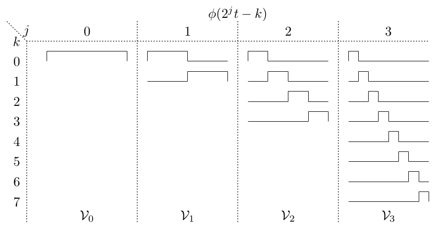
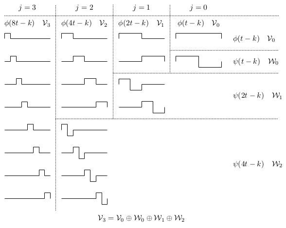
The Haar functions are illustrated in [link] where the first column contains thesimple constant basis function that spans , the second column contains the unit pulse of width one half and the one translate necessaryto span . The third column contains four translations of a pulse of width one fourth and the fourth contains eight translations of apulse of width one eighth. This shows clearly how increasing the scale allows greater and greater detail to be realized.However, using only the scaling function does not allow the decomposition described in the introduction. For that we need the wavelet. Rather thanuse the scaling functions in , we will use the orthogonal decomposition
which is the same as
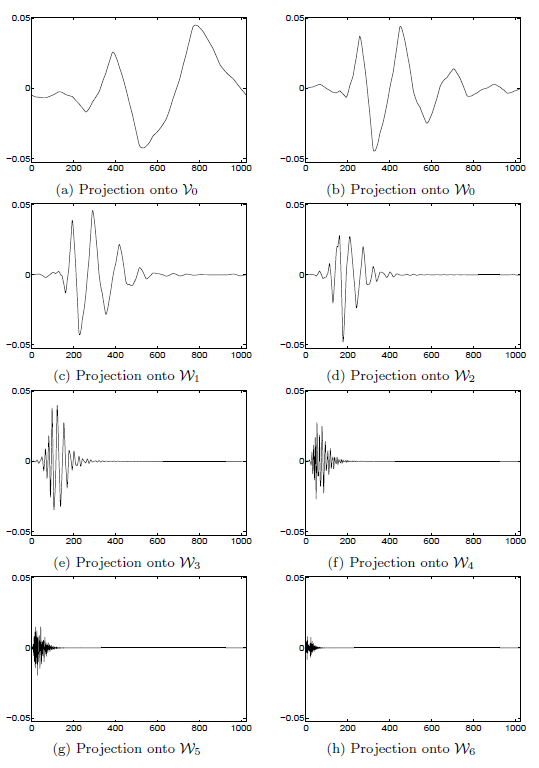
which means there are two sets of orthogonal basis functions that span , one in terms of scaling functions, and the other in terms of half as many coarser scaling functions plus the details contained in the wavelets. This is illustrated in [link] .
The can be further decomposed into
which is the same as
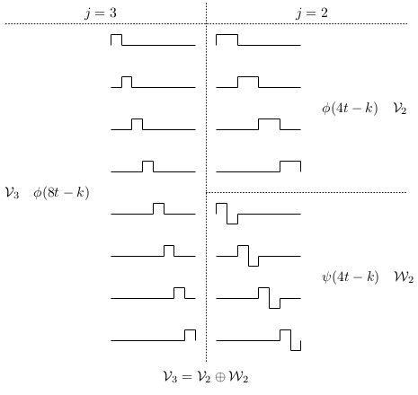
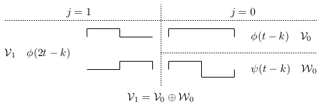
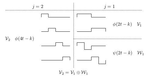
and this is illustrated in [link] . This gives also to be decomposed as
which is shown in [link] . By continuing to decompose the space spanned by the scaling function untilthe space is one constant, the complete decomposition of is obtained. This is symbolically shown in [link] .
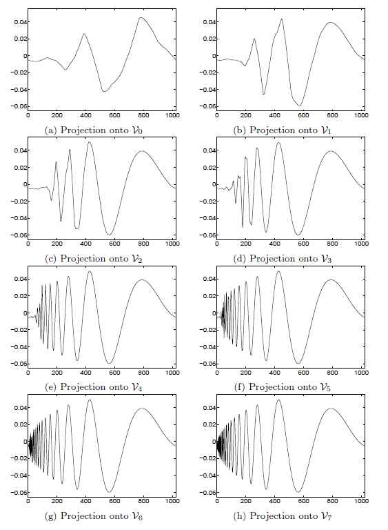
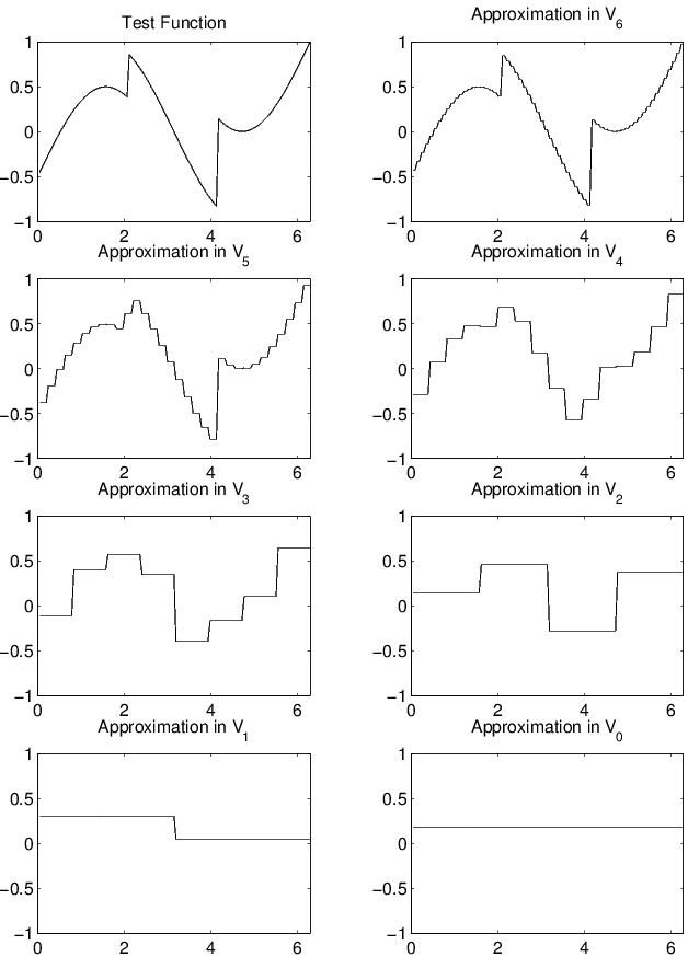
Finally we look at an approximation to a smooth function constructed from the basis elements in . Because the Haar functions form an orthogonal basis in each subspace, they can produce an optimal leastsquared error approximation to the smooth function. One can easily imagine the effects of adding a higher resolution “layer" of functions to giving an approximation residing in . Notice that these functions satisfy all of the conditions that we haveconsidered for scaling functions and wavelets. The basic wavelet is indeed an oscillating function which, in fact, has an average of zero andwhich will produce finer and finer detail as it is scaled and translated.
The multiresolution character of the scaling function and wavelet system is easily seen from [link] where a signal residing in can be expressed in terms of a sum of eight shifted scaling functions at scale or a sum of four shifted scaling functions and four shifted wavelets at a scale of . In the second case, the sum of four scaling functions gives a low resolution approximation to the signalwith the four wavelets giving the higher resolution “detail". The four shifted scaling functions could be further decomposed into coarser scalingfunctions and wavelets as illustrated in [link] and still further decomposed as shown in [link] .
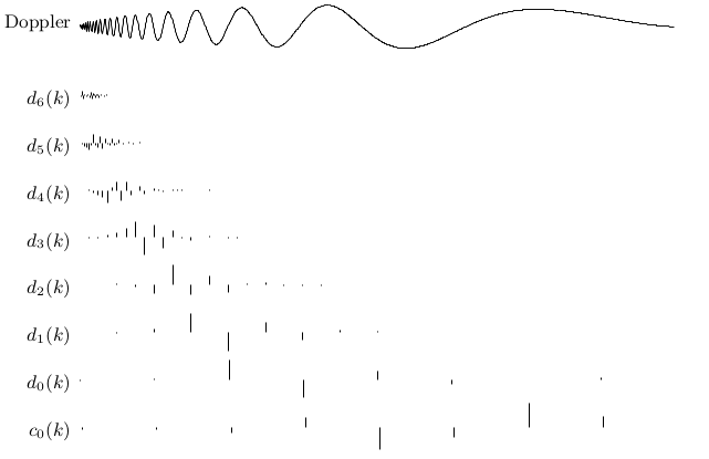
[link] shows the Haar approximations of a test function in various resolutions. The signal is an example of a mixture of a pure sinewave which would have a perfectly localized Fourier domain representation and a two discontinuities which are completely localized in time domain.The component at the coarsest scale is simply the average of the signal. As we include more and more wavelet scales, the approximation becomesclose to the original signal.
This chapter has skipped over some details in an attempt to communicate the general idea of the method. The conditions that can or must be satisfiedand the resulting properties, together with examples, are discussed in the following chapters and/or in the references.
Notification Switch
Would you like to follow the 'Wavelets and wavelet transforms' conversation and receive update notifications?
|
|

|
|

|
|

|
|
|
|
|

|
|

|
|

|
|

|
|

|