

| << Chapter < Page | Chapter >> Page > |
We have already explored some basic applications of exponential and logarithmic functions. In this section, we explore some important applications in more depth, including radioactive isotopes and Newton’s Law of Cooling.
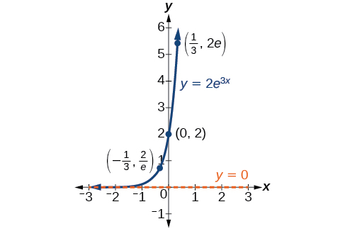
In real-world applications, we need to model the behavior of a function. In mathematical modeling, we choose a familiar general function with properties that suggest that it will model the real-world phenomenon we wish to analyze. In the case of rapid growth, we may choose the exponential growth function:
where is equal to the value at time zero, is Euler’s constant, and is a positive constant that determines the rate (percentage) of growth. We may use the exponential growth function in applications involving doubling time , the time it takes for a quantity to double. Such phenomena as wildlife populations, financial investments, biological samples, and natural resources may exhibit growth based on a doubling time. In some applications, however, as we will see when we discuss the logistic equation, the logistic model sometimes fits the data better than the exponential model.
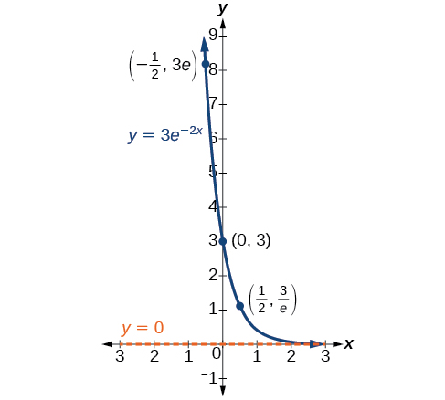
On the other hand, if a quantity is falling rapidly toward zero, without ever reaching zero, then we should probably choose the exponential decay model. Again, we have the form where is the starting value, and is Euler’s constant. Now is a negative constant that determines the rate of decay. We may use the exponential decay model when we are calculating half-life , or the time it takes for a substance to exponentially decay to half of its original quantity. We use half-life in applications involving radioactive isotopes.
In our choice of a function to serve as a mathematical model, we often use data points gathered by careful observation and measurement to construct points on a graph and hope we can recognize the shape of the graph. Exponential growth and decay graphs have a distinctive shape, as we can see in [link] and [link] . It is important to remember that, although parts of each of the two graphs seem to lie on the x -axis, they are really a tiny distance above the x -axis.
Exponential growth and decay often involve very large or very small numbers. To describe these numbers, we often use orders of magnitude. The order of magnitude is the power of ten, when the number is expressed in scientific notation, with one digit to the left of the decimal. For example, the distance to the nearest star, Proxima Centauri , measured in kilometers, is 40,113,497,200,000 kilometers. Expressed in scientific notation, this is So, we could describe this number as having order of magnitude
Notification Switch
Would you like to follow the 'Algebra and trigonometry' conversation and receive update notifications?

|
|

|
|

|
|

|
|

|
|
|
|
|

|
|

|
|

|
|

|
|
|
|