0.1 Proofs, identities, and toolkit functions

<< Chapter < Page

Algebra and trigonometry Page 1 / 1

Chapter >> Page >

Appendix

Important proofs and derivations

Product Rule

$\log_{a} x y = \log_{a} x + \log_{a} y$

Proof:

Let $m = \log_{a} x$ and $n = \log_{a} y .$

Write in exponent form.

$x = a^{m}$ and $y = a^{n} .$

Multiply.

$x y = a^{m} a^{n} = a^{m + n}$

$\begin{matrix} a^{m + n} & = & x y \\ \log_{a} (x y) & = & m + n \\ = & \log_{a} x + \log_{b} y \end{matrix}$

Change of Base Rule

$\begin{array}{l} \log_{a} b = \frac{\log_{c} b}{\log_{c} a} \\ \log_{a} b = \frac{1}{\log_{b} a} \end{array}$

where $x$ and $y$ are positive, and $a > 0, a \neq 1.$

Proof:

Let $x = \log_{a} b .$

Write in exponent form.

$a^{x} = b$

Take the $\log_{c}$ of both sides.

$\begin{matrix} \log_{c} a^{x} & = & \log_{c} b \\ x \log_{c} a & = & \log_{c} b \\ x & = & \frac{\log_{c} b}{\log_{c} a} \\ \log_{a} b & = & \frac{\log_{c} b}{\log_{a} b} \end{matrix}$

When $c = b,$

$\log_{a} b = \frac{\log_{b} b}{\log_{b} a} = \frac{1}{\log_{b} a}$

Heron’s Formula

$A = \sqrt{s (s - a) (s - b) (s - c)}$

where $s = \frac{a + b + c}{2}$

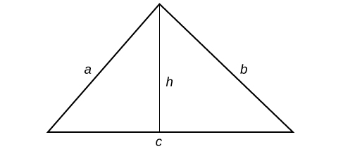
Proof:

Let $a,$ $b,$ and $c$ be the sides of a triangle, and $h$ be the height.

A triangle with sides labeled: a, b and c. A line runs through the center of the triangle, bisecting the top angle; this line is labeled: h.

So $s = \frac{a + b + c}{2}$ .

We can further name the parts of the base in each triangle established by the height such that $p + q = c .$

A triangle with sides labeled: a, b, and c. A line runs through the center of the triangle bisecting the angle at the top; this line is labeled: h. The two new line segments on the base of the triangle are labeled: p and q.

Using the Pythagorean Theorem, $h^{2} + p^{2} = a^{2}$ and $h^{2} + q^{2} = b^{2} .$

Since $q = c - p,$ then $q^{2} = {(c - p)}^{2} .$ Expanding, we find that $q^{2} = c^{2} - 2 c p + p^{2} .$

We can then add $h^{2}$ to each side of the equation to get $h^{2} + q^{2} = h^{2} + c^{2} - 2 c p + p^{2} .$

Substitute this result into the equation $h^{2} + q^{2} = b^{2}$ yields $b^{2} = h^{2} + c^{2} - 2 c p + p^{2} .$

Then replacing $h^{2} + p^{2}$ with $a^{2}$ gives $b^{2} = a^{2} - 2 c p + c^{2} .$

Solve for $p$ to get

$p = \frac{a^{2} + b^{2} - c^{2}}{2 c}$

Since $h^{2} = a^{2} - p^{2},$ we get an expression in terms of $a,$ $b,$ and $c .$

$\begin{matrix} h^{2} & = & a^{2} - p^{2} \\ = & (a + p) (a - p) \\ = & [a + \frac{(a^{2} + c^{2} - b^{2})}{2 c}] [a - \frac{(a^{2} + c^{2} - b^{2})}{2 c}] \\ = & \frac{(2 a c + a^{2} + c^{2} - b^{2}) (2 a c - a^{2} - c^{2} + b^{2})}{4 c^{2}} \\ = & \frac{({(a + c)}^{2} - b^{2}) (b^{2} - {(a - c)}^{2})}{4 c^{2}} \\ = & \frac{(a + b + c) (a + c - b) (b + a - c) (b - a + c)}{4 c^{2}} \\ = & \frac{(a + b + c) (- a + b + c) (a - b + c) (a + b - c)}{4 c^{2}} \\ = & \frac{2 s \cdot (2 s - a) \cdot (2 s - b) (2 s - c)}{4 c^{2}} \end{matrix}$

Therefore,

$\begin{matrix} h^{2} & = & \frac{4 s (s - a) (s - b) (s - c)}{c^{2}} \\ h & = & \frac{2 \sqrt{s (s - a) (s - b) (s - c)}}{c} \end{matrix}$

And since $A = \frac{1}{2} c h,$ then

$\begin{matrix} A & = & \frac{1}{2} c \frac{2 \sqrt{s (s - a) (s - b) (s - c)}}{c} \\ = & \sqrt{s (s - a) (s - b) (s - c)} \end{matrix}$

Properties of the Dot Product

$u \cdot v = v \cdot u$

Proof:

$\begin{matrix} u \cdot v & = ⟨ u_{1}, u_{2}, ... u_{n} ⟩ \cdot ⟨ v_{1}, v_{2}, ... v_{n} ⟩ \\ = u_{1} v_{1} + u_{2} v_{2} + ... + u_{n} v_{n} \\ = v_{1} u_{1} + v_{2} u_{2} + ... + v_{n} v_{n} \\ = ⟨ v_{1}, v_{2}, ... v_{n} ⟩ \cdot ⟨ u_{1}, u_{2}, ... u_{n} ⟩ \\ = v \cdot u \end{matrix}$

$u \cdot (v + w) = u \cdot v + u \cdot w$

Proof:

$\begin{matrix} u \cdot (v + w) & = ⟨ u_{1}, u_{2}, ... u_{n} ⟩ \cdot (⟨ v_{1}, v_{2}, ... v_{n} ⟩ + ⟨ w_{1}, w_{2}, ... w_{n} ⟩) \\ = ⟨ u_{1}, u_{2}, ... u_{n} ⟩ \cdot ⟨ v_{1} + w_{1}, v_{2} + w_{2}, ... v_{n} + w_{n} ⟩ \\ = ⟨ u_{1} (v_{1} + w_{1}), u_{2} (v_{2} + w_{2}), ... u_{n} (v_{n} + w_{n}) ⟩ \\ = ⟨ u_{1} v_{1} + u_{1} w_{1}, u_{2} v_{2} + u_{2} w_{2}, ... u_{n} v_{n} + u_{n} w_{n} ⟩ \\ = ⟨ u_{1} v_{1}, u_{2} v_{2}, ..., u_{n} v_{n} ⟩ + ⟨ u_{1} w_{1}, u_{2} w_{2}, ..., u_{n} w_{n} ⟩ \\ = ⟨ u_{1}, u_{2}, ... u_{n} ⟩ \cdot ⟨ v_{1}, v_{2}, ... v_{n} ⟩ + ⟨ u_{1}, u_{2}, ... u_{n} ⟩ \cdot ⟨ w_{1}, w_{2}, ... w_{n} ⟩ \\ = u \cdot v + u \cdot w \end{matrix}$

$u \cdot u = {| u |}^{2}$

Proof:

$\begin{matrix} u \cdot u & = ⟨ u_{1}, u_{2}, ... u_{n} ⟩ \cdot ⟨ u_{1}, u_{2}, ... u_{n} ⟩ \\ = u_{1} u_{1} + u_{2} u_{2} + ... + u_{n} u_{n} \\ = u_{1}^{2} + u_{2}^{2} + ... + u_{n}^{2} \\ = | ⟨ u_{1}, u_{2}, ... u_{n} ⟩ |^{2} \\ = v \cdot u \end{matrix}$

Standard Form of the Ellipse centered at the Origin

$1 = \frac{x^{2}}{a^{2}} + \frac{y^{2}}{b^{2}}$

Derivation

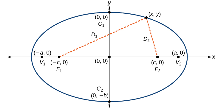
An ellipse consists of all the points for which the sum of distances from two foci is constant:

$\sqrt{{(x - (- c))}^{2} + {(y - 0)}^{2}} + \sqrt{{(x - c)}^{2} + {(y - 0)}^{2}} = constant$

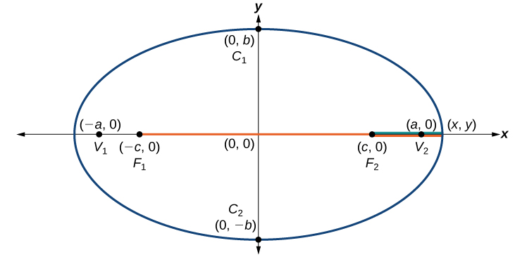
An ellipse centered at the origin on an x, y-coordinate plane. Points C1 and C2 are plotted at the points (0, b) and (0, -b) respectively; these points appear on the ellipse. Points V1 and V2 are plotted at the points (-a, 0) and (a, 0) respectively; these points appear on the ellipse. Points F1 and F2 are plotted at the points (-c, 0) and (c, 0) respectively; these points appear on the x-axis, but not the ellipse. The point (x, y) appears on the ellipse in the first quadrant. Dotted lines extend from F1 and F2 to the point (x, y).

Consider a vertex.

An ellipse centered at the origin. The points C1 and C2 are plotted at the points (0, b) and (0, -b) respectively; these points are on the ellipse. The points V1 and V2 are plotted at the points (-a, 0) and (a, 0) respectively; these points are on the ellipse. The points F1 and F2 are plotted at the points (-c, 0) and (c, 0) respectively; these points are on the x-axis and not on the ellipse. A line extends from the point F1 to a point (x, y) which is at the point (a, 0). A line extends from the point F2 to the point (x, y) as well.

Then, $\sqrt{{(x - (- c))}^{2} + {(y - 0)}^{2}} + \sqrt{{(x - c)}^{2} + {(y - 0)}^{2}} = 2 a$

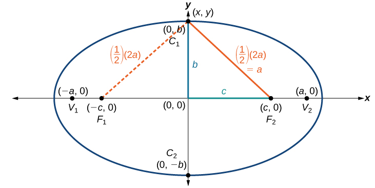
Consider a covertex.

Then $b^{2} + c^{2} = a^{2} .$

$\begin{matrix} \sqrt{{(x - (- c))}^{2} + {(y - 0)}^{2}} + \sqrt{{(x - c)}^{2} + {(y - 0)}^{2}} & = & 2 a \\ \sqrt{{(x + c)}^{2} + y^{2}} & = & 2 a - \sqrt{{(x - c)}^{2} + y^{2}} \\ {(x + c)}^{2} + y^{2} & = & {(2 a - \sqrt{{(x - c)}^{2} + y^{2}})}^{2} \\ x^{2} + 2 c x + c^{2} + y^{2} & = & 4 a^{2} - 4 a \sqrt{{(x - c)}^{2} + y^{2}} + {(x - c)}^{2} + y^{2} \\ x^{2} + 2 c x + c^{2} + y^{2} & = & 4 a^{2} - 4 a \sqrt{{(x - c)}^{2} + y^{2}} + x^{2} - 2 c x + y^{2} \\ 2 c x & = & 4 a^{2} - 4 a \sqrt{{(x - c)}^{2} + y^{2}} - 2 c x \\ 4 c x - 4 a^{2} & = & 4 a \sqrt{{(x - c)}^{2} + y^{2}} \\ - \frac{1}{4 a} (4 c x - 4 a^{2}) & = & \sqrt{{(x - c)}^{2} + y^{2}} \\ a - \frac{c}{a} x & = & \sqrt{{(x - c)}^{2} + y^{2}} \\ a^{2} - 2 x c + \frac{c^{2}}{a^{2}} x^{2} & = & {(x - c)}^{2} + y^{2} \\ a^{2} - 2 x c + \frac{c^{2}}{a^{2}} x^{2} & = & x^{2} - 2 x c + c^{2} + y^{2} \\ a^{2} + \frac{c^{2}}{a^{2}} x^{2} & = & x^{2} + c^{2} + y^{2} \\ a^{2} + \frac{c^{2}}{a^{2}} x^{2} & = & x^{2} + c^{2} + y^{2} \\ a^{2} - c^{2} & = & x^{2} - \frac{c^{2}}{a^{2}} x^{2} + y^{2} \\ a^{2} - c^{2} & = & x^{2} (1 - \frac{c^{2}}{a^{2}}) + y^{2} \end{matrix}$

Let $1 = \frac{a^{2}}{a^{2}} .$

\begin{matrix} a^{2} - c^{2} & = & x^{2} (\frac{a^{2} - c^{2}}{a^{2}}) + y^{2} \\ 1 & = & \frac{x^{2}}{a^{2}} + \frac{y^{2}}{a^{2} - c^{2}} \end{matrix}

Because $b^{2} + c^{2} = a^{2},$ then $b^{2} = a^{2} - c^{2} .$

\begin{matrix} 1 & = & \frac{x^{2}}{a^{2}} + \frac{y^{2}}{a^{2} - c^{2}} \\ 1 & = & \frac{x^{2}}{a^{2}} + \frac{y^{2}}{b^{2}} \end{matrix}

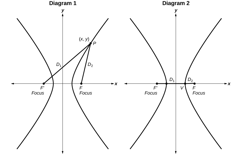
Standard Form of the Hyperbola

$1 = \frac{x^{2}}{a^{2}} - \frac{y^{2}}{b^{2}}$

Derivation

A hyperbola is the set of all points in a plane such that the absolute value of the difference of the distances between two fixed points is constant.

Side-by-side graphs of hyperbole. In Diagram 1: The foci F’ and F are labeled and can be found a little in front of the opening of the hyperbola. A point P at (x,y) on the right curve is labeled. A line extends from the F’ focus to the point P labeled: D1. A line extends from the F focus to the point P labeled: D2. In Diagram 2: The foci F’ and F are labeled and can be found a little in front of the opening of the hyperbola. A point V is labeled at the vertex of the right hyperbola. A line extends from the F’ focus to the point V labeled: D1. A line extends from the F focus to the point V labeled: D2.

Diagram 1: The difference of the distances from Point P to the foci is constant:

$\sqrt{{(x - (- c))}^{2} + {(y - 0)}^{2}} - \sqrt{{(x - c)}^{2} + {(y - 0)}^{2}} = constant$

Diagram 2: When the point is a vertex, the difference is $2 a .$

$\sqrt{{(x - (- c))}^{2} + {(y - 0)}^{2}} - \sqrt{{(x - c)}^{2} + {(y - 0)}^{2}} = 2 a$

$\begin{matrix} \sqrt{{(x - (- c))}^{2} + {(y - 0)}^{2}} - \sqrt{{(x - c)}^{2} + {(y - 0)}^{2}} & = & 2 a \\ \sqrt{{(x + c)}^{2} + y^{2}} - \sqrt{{(x - c)}^{2} + y^{2}} & = & 2 a \\ \sqrt{{(x + c)}^{2} + y^{2}} & = & 2 a + \sqrt{{(x - c)}^{2} + y^{2}} \\ {(x + c)}^{2} + y^{2} & = & (2 a + \sqrt{{(x - c)}^{2} + y^{2}}) \\ x^{2} + 2 c x + c^{2} + y^{2} & = & 4 a^{2} + 4 a \sqrt{{(x - c)}^{2}} + y^{2} \\ x^{2} + 2 c x + c^{2} + y^{2} & = & 4 a^{2} + 4 a \sqrt{{(x - c)}^{2} + y^{2}} + x^{2} - 2 c x + y^{2} \\ 2 c x & = & 4 a^{2} + 4 a \sqrt{{(x - c)}^{2} + y^{2}} - 2 c x \\ 4 c x - 4 a^{2} & = & 4 a \sqrt{{(x - c)}^{2} + y^{2}} \\ c x - a^{2} & = & a \sqrt{{(x - c)}^{2} + y^{2}} \\ {(c x - a^{2})}^{2} & = & a^{2} ({(x - c)}^{2} + y^{2}) \\ c^{2} x^{2} - 2 a^{2} c^{2} x^{2} + a^{4} & = & a^{2} x^{2} - 2 a^{2} c^{2} x^{2} + a^{2} c^{2} + a^{2} y^{2} \\ c^{2} x^{2} + a^{4} & = & a^{2} x^{2} + a^{2} c^{2} + a^{2} y^{2} \\ a^{4} - a^{2} c^{2} & = & a^{2} x^{2} - c^{2} x^{2} + a^{2} y^{2} \\ a^{2} (a^{2} - c^{2}) & = & (a^{2} - c^{2}) x^{2} + a^{2} y^{2} \\ a^{2} (a^{2} - c^{2}) & = & (c^{2} - a^{2}) x^{2} - a^{2} y^{2} \end{matrix}$

Define $b$ as a positive number such that $b^{2} = c^{2} - a^{2} .$

\begin{matrix} a^{2} b^{2} & = & b^{2} x^{2} - a^{2} y^{2} \\ \frac{a^{2} b^{2}}{a^{2} b^{2}} & = & \frac{b^{2} x^{2}}{a^{2} b^{2}} - \frac{a^{2} y^{2}}{a^{2} b^{2}} \\ 1 & = & \frac{x^{2}}{a^{2}} - \frac{y^{2}}{b^{2}} \end{matrix}

Trigonometric identities

Pythagorean Identity	$\begin{array}{l} \cos^{2} t + \sin^{2} t = 1 \\ 1 + \tan^{2} t = \sec^{2} t \\ 1 + \cot^{2} t = \csc^{2} t \end{array}$
Even-Odd Identities	$\begin{array}{l} \cos (- t) = c o s t \\ \sec (- t) = \sec t \\ \sin (- t) = - \sin t \\ \tan (- t) = - \tan t \\ \csc (- t) = - \csc t \\ \cot (- t) = - \cot t \end{array}$
Cofunction Identities	$\begin{array}{l} \cos t = \sin (\frac{π}{2} - t) \\ \sin t = \cos (\frac{π}{2} - t) \\ \tan t = \cot (\frac{π}{2} - t) \\ \cot t = \tan (\frac{π}{2} - t) \\ \sec t = \csc (\frac{π}{2} - t) \\ \csc t = \sec (\frac{π}{2} - t) \end{array}$
Fundamental Identities	$\begin{array}{l} \tan t = \frac{\sin t}{\cos t} \\ \sec t = \frac{1}{\cos t} \\ \csc t = \frac{1}{\sin t} \\ c o t t = \frac{1}{tan t} = \frac{cos t}{sin t} \end{array}$
Sum and Difference Identities	$\begin{array}{l} \cos (α + β) = \cos α \cos β - \sin α \sin β \\ \cos (α - β) = \cos α \cos β + \sin α \sin β \\ \sin (α + β) = \sin α \cos β + \cos α \sin β \\ \sin (α - β) = \sin α \cos β - \cos α \sin β \\ \tan (α + β) = \frac{\tan α + \tan β}{1 - \tan α \tan β} \\ \tan (α - β) = \frac{\tan α - \tan β}{1 + \tan α \tan β} \end{array}$
Double-Angle Formulas	$\begin{array}{l} \sin (2 θ) = 2 \sin θ \cos θ \\ \cos (2 θ) = \cos^{2} θ - \sin^{2} θ \\ \cos (2 θ) = 1 - 2 \sin^{2} θ \\ \cos (2 θ) = 2 \cos^{2} θ - 1 \\ \tan (2 θ) = \frac{2 \tan θ}{1 - \tan^{2} θ} \end{array}$
Half-Angle Formulas	$\begin{array}{l} \sin \frac{α}{2} = \pm \sqrt{\frac{1 - \cos α}{2}} \\ \cos \frac{α}{2} = \pm \sqrt{\frac{1 + \cos α}{2}} \\ \tan \frac{α}{2} = \pm \sqrt{\frac{1 - \cos α}{1 + \cos α}} \\ \tan \frac{α}{2} = \frac{\sin α}{1 + \cos α} \\ \tan \frac{α}{2} = \frac{1 - \cos α}{\sin α} \end{array}$
Reduction Formulas	$\begin{array}{l} \sin^{2} θ = \frac{1 - \cos (2 θ)}{2} \\ \cos^{2} θ = \frac{1 + \cos (2 θ)}{2} \\ \tan^{2} θ = \frac{1 - \cos (2 θ)}{1 + \cos (2 θ)} \end{array}$
Product-to-Sum Formulas	$\begin{array}{l} \cos α \cos β = \frac{1}{2} [\cos (α - β) + \cos (α + β)] \\ \sin α \cos β = \frac{1}{2} [\sin (α + β) + \sin (α - β)] \\ \sin α \sin β = \frac{1}{2} [\cos (α - β) - \cos (α + β)] \\ \cos α \sin β = \frac{1}{2} [\sin (α + β) - \sin (α - β)] \end{array}$
Sum-to-Product Formulas	$\begin{array}{l} \sin α + \sin β = 2 \sin (\frac{α + β}{2}) \cos (\frac{α - β}{2}) \\ \sin α - \sin β = 2 \sin (\frac{α - β}{2}) \cos (\frac{α + β}{2}) \\ \cos α - \cos β = - 2 \sin (\frac{α + β}{2}) \sin (\frac{α - β}{2}) \\ \cos α + \cos β = 2 \cos (\frac{α + β}{2}) \cos (\frac{α - β}{2}) \end{array}$
Law of Sines	$\begin{array}{l} \frac{\sin α}{a} = \frac{\sin β}{b} = \frac{\sin γ}{c} \\ \frac{a}{\sin α} = \frac{b}{\sin β} = \frac{c}{\sin γ} \end{array}$
Law of Cosines	$\begin{matrix} a^{2} = b^{2} + c^{2} - 2 b c \cos α \\ b^{2} = a^{2} + c^{2} - 2 a c \cos β \\ c^{2} = a^{2} + b^{2} - 2 a b cos γ \end{matrix}$

Toolkit functions

Three graphs side-by-side. From left to right, graph of the identify function, square function, and square root function. All three graphs extend from -4 to 4 on each axis.

Three graphs side-by-side. From left to right, graph of the cubic function, cube root function, and reciprocal function. All three graphs extend from -4 to 4 on each axis.

Three graphs side-by-side. From left to right, graph of the absolute value function, exponential function, and natural logarithm function. All three graphs extend from -4 to 4 on each axis.

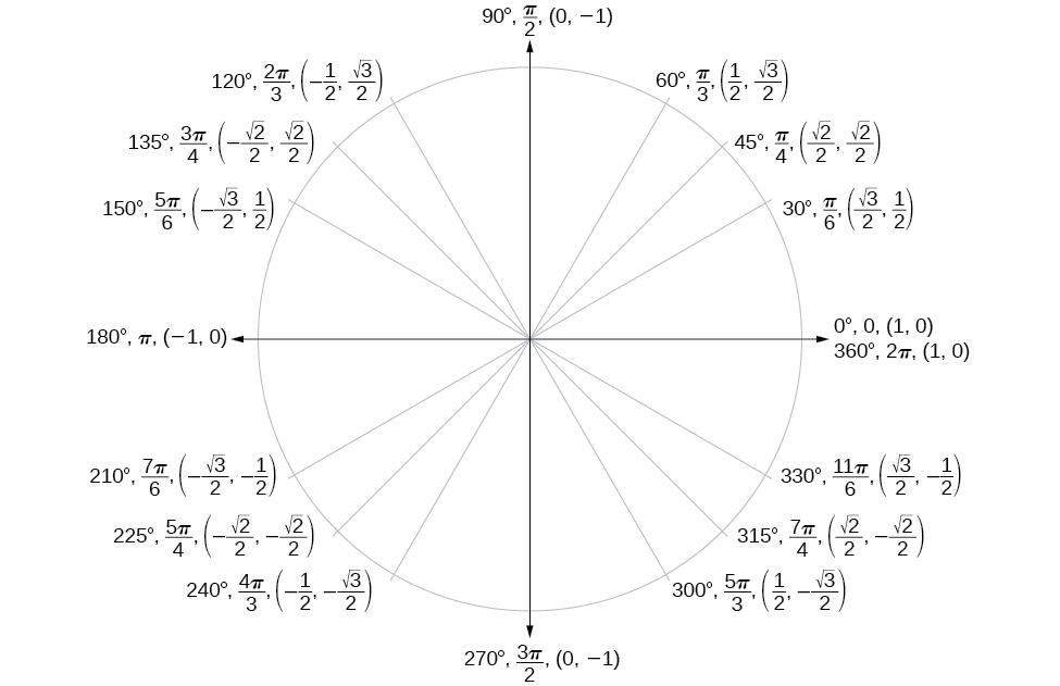
Trigonometric functions

Unit Circle

Angle	$0$	$\frac{π}{6}, or 30 °$	$\frac{π}{4}, or 45 °$	$\frac{π}{3}, or 60 °$	$\frac{π}{2}, or 90 °$
Cosine	1	$\frac{\sqrt{3}}{2}$	$\frac{\sqrt{2}}{2}$	$\frac{1}{2}$	0
Sine	0	$\frac{1}{2}$	$\frac{\sqrt{2}}{2}$	$\frac{\sqrt{3}}{2}$	1
Tangent	0	$\frac{\sqrt{3}}{3}$	1	$\sqrt{3}$	Undefined
Secant	1	$\frac{2 \sqrt{3}}{3}$	$\sqrt{2}$	2	Undefined
Cosecant	Undefined	2	$\sqrt{2}$	$\frac{2 \sqrt{3}}{3}$	1
Cotangent	Undefined	$\sqrt{3}$	1	$\frac{\sqrt{3}}{3}$	0

Questions & Answers

Ayele, K., 2003. Introductory Economics, 3rd ed., Addis Ababa.

Widad Reply

can you send the book attached ?

Ariel

What is economics

Widad Reply

the study of how humans make choices under conditions of scarcity

AI-Robot

U(x,y) = (x×y)1/2 find mu of x for y

Desalegn Reply

U(x,y) = (xÃy)1/2 find mu of x for y

Desalegn

what is ecnomics

Jan Reply

this is the study of how the society manages it's scarce resources

Belonwu

what is macroeconomic

John Reply

macroeconomic is the branch of economics which studies actions, scale, activities and behaviour of the aggregate economy as a whole.

husaini

etc

husaini

difference between firm and industry

husaini Reply

what's the difference between a firm and an industry

Abdul

firm is the unit which transform inputs to output where as industry contain combination of firms with similar production 😅😅

Abdulraufu

Suppose the demand function that a firm faces shifted from Qd  120 3P to Qd  90  3P and the supply function has shifted from QS  20  2P to QS 10  2P . a) Find the effect of this change on price and quantity. b) Which of the changes in demand and supply is higher?

Toofiq Reply

explain standard reason why economic is a science

innocent Reply

factors influencing supply

Petrus Reply

what is economic.

Milan Reply

scares means__________________ends resources. unlimited

Jan

economics is a science that studies human behaviour as a relationship b/w ends and scares means which have alternative uses

Jan

calculate the profit maximizing for demand and supply

Zarshad Reply

Why qualify 28 supplies

Milan

what are explicit costs

Nomsa Reply

out-of-pocket costs for a firm, for example, payments for wages and salaries, rent, or materials

AI-Robot

concepts of supply in microeconomics

David Reply

economic overview notes

Amahle Reply

identify a demand and a supply curve

Salome Reply

i don't know

Parul

there's a difference

Aryan

Demand curve shows that how supply and others conditions affect on demand of a particular thing and what percent demand increase whith increase of supply of goods

Israr

Hi Sir please how do u calculate Cross elastic demand and income elastic demand?

Abari

Got questions? Join the online conversation and get instant answers!

Jobilize.com Reply

<< Chapter < Page Page > Chapter >>

Read also:

Get Jobilize Job Search Mobile App in your pocket Now!

100% Free Mobile Applications
Receive real-time job alerts and never miss the right job again

Source: OpenStax, Algebra and trigonometry. OpenStax CNX. Nov 14, 2016 Download for free at https://legacy.cnx.org/content/col11758/1.6

Google Play and the Google Play logo are trademarks of Google Inc.

Notification Switch

Would you like to follow the 'Algebra and trigonometry' conversation and receive update notifications?

Ask

	13 Dr Garry GI Ruminants quiz By Brooke Delaney Start Exam
	34 Biology 34 Animal Nutrition Digestive System By OpenStax Start Quiz
	Anthropology Religion Culture By Richley Crapo Start Assignment
	16 Biology 16 Gene Expression MCQ By OpenStax Start Quiz
	9 AP 09 Joints MCQ Quiz By OpenStax Start Quiz
	Immunology Practice Test By Sandhills MLT Start Test
	Does your crush like you? By Hoy Wen Start Quiz
	39 Biology 39 The Respiratory System MCQ By OpenStax Start Quiz
	Social Organization Kinship By Richley Crapo Start Assignment
	World Capitals Quiz By Yasser Ibrahim Start Quiz