2.7 Measures of the spread of the data  (Page 6/25)

Standard deviation of grouped frequency tables

Recall that for grouped data we do not know individual data values, so we cannot describe the typical value of the data with precision. In other words, we cannot find the exact mean, median, or mode. We can, however, determine the best estimate of the measures of center by finding the mean of the grouped data with the formula: $MeanofFrequencyTable=\frac{{\displaystyle \sum fm}}{{\displaystyle \sum f}}$
where $f=$ interval frequencies and m = interval midpoints.

Just as we could not find the exact mean, neither can we find the exact standard deviation. Remember that standard deviation describes numerically the expected deviation a data value has from the mean. In simple English, the standard deviation allows us to compare how “unusual” individual data is compared to the mean.

Try it

Find the standard deviation for the data from the previous example

Class	Frequency, f
0–2	1
3–5	6
6–8	10
9–11	7
12–14	0
15–17	2

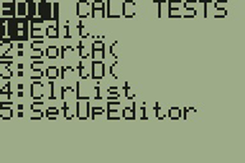
First, press the STAT key and select 1:Edit

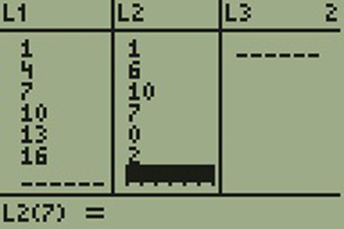
Input the midpoint values into L1 and the frequencies into L2

Select STAT , CALC , and 1: 1-Var Stats

Select 2 ^nd then 1 then , 2 ^nd then 2 Enter

You will see displayed both a population standard deviation, σ _x , and the sample standard deviation, s _x .

Comparing values from different data sets

The standard deviation is useful when comparing data values that come from different data sets. If the data sets have different means and standard deviations, then comparing the data values directly can be misleading.

• For each data value, calculate how many standard deviations away from its mean the value is.
• Use the formula: value = mean + (#ofSTDEVs)(standard deviation); solve for #ofSTDEVs.
• $\#ofSTDEVs=\frac{\text{value – mean}}{\text{standard deviation}}$
• Compare the results of this calculation.