<< Chapter < Page Chapter >> Page >
The image shows radish plants of various heights sprouting out of dirt.
The heights of these radish plants are continuous random variables. (Credit: Rev Stan)

Chapter objectives

By the end of this chapter, the student should be able to:

  • Recognize and understand continuous probability density functions in general.
  • Recognize the uniform probability distribution and apply it appropriately.
  • Recognize the exponential probability distribution and apply it appropriately.

Continuous random variables have many applications. Baseball batting averages, IQ scores, the length of time a long distance telephone call lasts, the amount of money a person carries, the length of time a computer chip lasts, and SAT scores are just a few. The field of reliability depends on a variety of continuous random variables.

Note

The values of discrete and continuous random variables can be ambiguous. For example, if X is equal to the number of miles (to the nearest mile) you drive to work, then X is a discrete random variable. You count the miles. If X is the distance you drive to work, then you measure values of X and X is a continuous random variable. For a second example, if X is equal to the number of books in a backpack, then X is a discrete random variable. If X is the weight of a book, then X is a continuous random variable because weights are measured. How the random variable is defined is very important.

Properties of continuous probability distributions

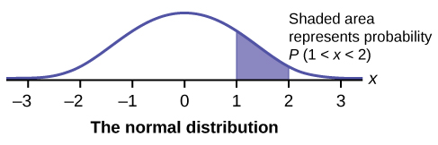
The graph of a continuous probability distribution is a curve. Probability is represented by area under the curve.

The curve is called the probability density function (abbreviated as pdf ). We use the symbol f ( x ) to represent the curve. f ( x ) is the function that corresponds to the graph; we use the density function f ( x ) to draw the graph of the probability distribution.

Area under the curve is given by a different function called the cumulative distribution function (abbreviated as cdf ). The cumulative distribution function is used to evaluate probability as area.

  • The outcomes are measured, not counted.
  • The entire area under the curve and above the x-axis is equal to one.
  • Probability is found for intervals of x values rather than for individual x values.
  • P(c<x<d) is the probability that the random variable X is in the interval between the values c and d . P(c<x<d) is the area under the curve, above the x -axis, to the right of c and the left of d .
  • P(x = c) = 0 The probability that x takes on any single individual value is zero. The area below the curve, above the x -axis, and between x = c and x = c has no width, and therefore no area (area = 0). Since the probability is equal to the area, the probability is also zero.
  • P(c<x<d) is the same as P(c ≤ x ≤ d) because probability is equal to area.

We will find the area that represents probability by using geometry, formulas, technology, or probability tables. In general, calculus is needed to find the area under the curve for many probability density functions. When we use formulas to find the area in this textbook, the formulas were found by using the techniques of integral calculus. However, because most students taking this course have not studied calculus, we will not be using calculus in this textbook.

There are many continuous probability distributions. When using a continuous probability distribution to model probability, the distribution used is selected to model and fit the particular situation in the best way.

In this chapter and the next, we will study the uniform distribution, the exponential distribution, and the normal distribution. The following graphs illustrate these distributions.

This graph shows a uniform distribution. The horizontal axis ranges from 0 to 10. The distribution is modeled by a rectangle extending from x = 2 to x = 8.8. A region from x = 3 to x = 6 is shaded inside the rectangle. The shaded area represents P(3  x < 6).
The graph shows a Uniform Distribution with the area between x = 3 and x = 6 shaded to represent the probability that the value of the random variable X is in the interval between three and six.
The graph shows an Exponential Distribution with the area between x = 2 and x = 4 shaded to represent the probability that the value of the random variable X is in the interval between two and four.
This graph shows an exponential distribution. The graph slopes downward. It begins at a point on the y-axis and approaches the x-axis at the right edge of the graph. The region under the graph from x = 2 to x = 4 is shaded to represent P(2 < x < 4).
The graph shows the Standard Normal Distribution with the area between x = 1 and x = 2 shaded to represent the probability that the value of the random variable X is in the interval between one and two.

Questions & Answers

how do you get the 2/50
Abba Reply
number of sport play by 50 student construct discrete data
Aminu Reply
width of the frangebany leaves on how to write a introduction
Theresa Reply
Solve the mean of variance
Veronica Reply
Step 1: Find the mean. To find the mean, add up all the scores, then divide them by the number of scores. ... Step 2: Find each score's deviation from the mean. ... Step 3: Square each deviation from the mean. ... Step 4: Find the sum of squares. ... Step 5: Divide the sum of squares by n – 1 or N.
kenneth
what is error
Yakuba Reply
Is mistake done to something
Vutshila
Hy
anas
hy
What is the life teble
anas
hy
Jibrin
statistics is the analyzing of data
Tajudeen Reply
what is statics?
Zelalem Reply
how do you calculate mean
Gloria Reply
diveving the sum if all values
Shaynaynay
let A1,A2 and A3 events be independent,show that (A1)^c, (A2)^c and (A3)^c are independent?
Fisaye Reply
what is statistics
Akhisani Reply
data collected all over the world
Shaynaynay
construct a less than and more than table
Imad Reply
The sample of 16 students is taken. The average age in the sample was 22 years with astandard deviation of 6 years. Construct a 95% confidence interval for the age of the population.
Aschalew Reply
Bhartdarshan' is an internet-based travel agency wherein customer can see videos of the cities they plant to visit. The number of hits daily is a normally distributed random variable with a mean of 10,000 and a standard deviation of 2,400 a. what is the probability of getting more than 12,000 hits? b. what is the probability of getting fewer than 9,000 hits?
Akshay Reply
Bhartdarshan'is an internet-based travel agency wherein customer can see videos of the cities they plan to visit. The number of hits daily is a normally distributed random variable with a mean of 10,000 and a standard deviation of 2,400. a. What is the probability of getting more than 12,000 hits
Akshay
1
Bright
Sorry i want to learn more about this question
Bright
Someone help
Bright
a= 0.20233 b=0.3384
Sufiyan
a
Shaynaynay
How do I interpret level of significance?
Mohd Reply
It depends on your business problem or in Machine Learning you could use ROC- AUC cruve to decide the threshold value
Shivam
how skewness and kurtosis are used in statistics
Owen Reply
yes what is it
Taneeya
Practice Key Terms 2

Get Jobilize Job Search Mobile App in your pocket Now!

Get it on Google Play Download on the App Store Now


Source:  OpenStax, Introductory statistics. OpenStax CNX. May 06, 2016 Download for free at http://legacy.cnx.org/content/col11562/1.18
Google Play and the Google Play logo are trademarks of Google Inc.

Notification Switch

Would you like to follow the 'Introductory statistics' conversation and receive update notifications?

Ask