

| << Chapter < Page | Chapter >> Page > |
Identify the potential outlier in the scatter plot. The standard deviation of the residuals or errors is approximately 8.6.
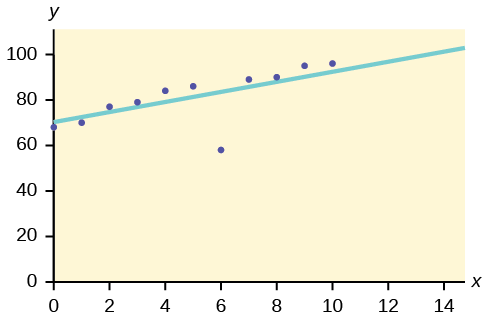
The outlier appears to be at (6, 58). The expected y value on the line for the point (6, 58) is approximately 82. Fifty-eight is 24 units from 82. Twenty-four is more than two standard deviations (2 s = (2)(8.6) = 17.2 ). So 82 is more than two standard deviations from 58, which makes (6, 58) a potential outlier.
In [link] , the first two columns are the third-exam and final-exam data. The third column shows the predicted ŷ values calculated from the line of best fit: ŷ = –173.5 + 4.83 x . The residuals, or errors, have been calculated in the fourth column of the table: observed y value−predicted y value = y − ŷ .
s is the standard deviation of all the y − ŷ = ε values where n = the total number of data points. If each residual is calculated and squared, and the results are added, we get the SSE. The standard deviation of the residuals is calculated from the SSE as:
We divide by ( n – 2) because the regression model involves two estimates.
Rather than calculate the value of s ourselves, we can find s using the computer or calculator. For this example, the calculator function LinRegTTest found s = 16.4 as the standard deviation of the residuals
| x | y | ŷ | y – ŷ |
|---|---|---|---|
| 65 | 175 | 140 | 175 – 140 = 35 |
| 67 | 133 | 150 | 133 – 150= –17 |
| 71 | 185 | 169 | 185 – 169 = 16 |
| 71 | 163 | 169 | 163 – 169 = –6 |
| 66 | 126 | 145 | 126 – 145 = –19 |
| 75 | 198 | 189 | 198 – 189 = 9 |
| 67 | 153 | 150 | 153 – 150 = 3 |
| 70 | 163 | 164 | 163 – 164 = –1 |
| 71 | 159 | 169 | 159 – 169 = –10 |
| 69 | 151 | 160 | 151 – 160 = –9 |
| 69 | 159 | 160 | 159 – 160 = –1 |
We are looking for all data points for which the residual is greater than 2 s = 2(16.4) = 32.8 or less than –32.8. Compare these values to the residuals in column four of the table. The only such data point is the student who had a grade of 65 on the third exam and 175 on the final exam; the residual for this student is 35.
Numerically and graphically, we have identified the point (65, 175) as an outlier. We should re-examine the data for this point to see if there are any problems with the data. If there is an error, we should fix the error if possible, or delete the data. If the data is correct, we would leave it in the data set. For this problem, we will suppose that we examined the data and found that this outlier data was an error. Therefore we will continue on and delete the outlier, so that we can explore how it affects the results, as a learning experience.
ŷ = –355.19 + 7.39 x and r = 0.9121
The new line with r = 0.9121 is a stronger correlation than the original ( r = 0.6631) because r = 0.9121 is closer to one. This means that the new line is a better fit to the ten remaining data values. The line can better predict the final exam score given the third exam score.
Notification Switch
Would you like to follow the 'Introductory statistics' conversation and receive update notifications?

|
|
|
|
|

|
|

|
|

|
|

|
|

|
|

|
|

|
|

|
|
|
|
|

|