<< Chapter < Page Chapter >> Page >

In some data sets, there are values (observed data points) called outliers . Outliers are observed data points that are far from the least squares line. They have large "errors", where the "error" or residual is the vertical distance from the line to the point.

Outliers need to be examined closely. Sometimes, for some reason or another, they should not be included in the analysis of the data. It is possible that an outlier is a result of erroneous data. Other times, an outlier may hold valuable information about the population under study and should remain included in the data. The key is to examine carefully what causes a data point to be an outlier.

Besides outliers, a sample may contain one or a few points that are called influential points . Influential points are observed data points that are far from the other observed data points in the horizontal direction. These points may have a big effect on the slope of the regression line. To begin to identify an influential point, you can remove it from the data set and see if the slope of the regression line is changed significantly.

Computers and many calculators can be used to identify outliers from the data. Computer output for regression analysis will often identify both outliers and influential points so that you can examine them.

Identifying outliers

We could guess at outliers by looking at a graph of the scatterplot and best fit-line. However, we would like some guideline as to how far away a point needs to be in order to be considered an outlier. As a rough rule of thumb, we can flag any point that is located further than two standard deviations above or below the best-fit line as an outlier . The standard deviation used is the standard deviation of the residuals or errors.

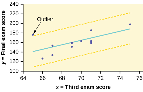
We can do this visually in the scatter plot by drawing an extra pair of lines that are two standard deviations above and below the best-fit line. Any data points that are outside this extra pair of lines are flagged as potential outliers. Or we can do this numerically by calculating each residual and comparing it to twice the standard deviation. On the TI-83, 83+, or 84+, the graphical approach is easier. The graphical procedure is shown first, followed by the numerical calculations. You would generally need to use only one of these methods.

In the third exam/final exam example , you can determine if there is an outlier or not. If there is an outlier, as an exercise, delete it and fit the remaining data to a new line. For this example, the new line ought to fit the remaining data better. This means the SSE should be smaller and the correlation coefficient ought to be closer to 1 or –1.

Graphical identification of outliers

With the TI-83, 83+, 84+ graphing calculators, it is easy to identify the outliers graphically and visually. If we were to measure the vertical distance from any data point to the corresponding point on the line of best fit and that distance were equal to 2 s or more, then we would consider the data point to be "too far" from the line of best fit. We need to find and graph the lines that are two standard deviations below and above the regression line. Any points that are outside these two lines are outliers. We will call these lines Y2 and Y3:

As we did with the equation of the regression line and the correlation coefficient, we will use technology to calculate this standard deviation for us. Using the LinRegTTest with this data, scroll down through the output screens to find s = 16.412 .

Line Y2 = –173.5 + 4.83 x –2(16.4) and line Y3 = –173.5 + 4.83 x + 2(16.4)

where ŷ = –173.5 + 4.83 x is the line of best fit. Y2 and Y3 have the same slope as the line of best fit.

Graph the scatterplot with the best fit line in equation Y1, then enter the two extra lines as Y2 and Y3 in the "Y="equation editor and press ZOOM 9. You will find that the only data point that is not between lines Y2 and Y3 is the point x = 65, y = 175. On the calculator screen it is just barely outside these lines. The outlier is the student who had a grade of 65 on the third exam and 175 on the final exam; this point is further than two standard deviations away from the best-fit line.

Sometimes a point is so close to the lines used to flag outliers on the graph that it is difficult to tell if the point is between or outside the lines. On a computer, enlarging the graph may help; on a small calculator screen, zooming in may make the graph clearer. Note that when the graph does not give a clear enough picture, you can use the numerical comparisons to identify outliers.

The scatter plot of exam scores with a line of best fit.Two yellow dashed lines run parallel to the line of best fit. The dashed lines run above and below the best fit line at equal distances. One data point falls outside the boundary created by the dashed lines—it is an outlier.
Got questions? Get instant answers now!

Questions & Answers

What are the factors that affect demand for a commodity
Florence Reply
differentiate between demand and supply giving examples
Lambiv Reply
differentiated between demand and supply using examples
Lambiv
what is labour ?
Lambiv
how will I do?
Venny Reply
how is the graph works?I don't fully understand
Rezat Reply
information
Eliyee
devaluation
Eliyee
t
WARKISA
hi guys good evening to all
Lambiv
multiple choice question
Aster Reply
appreciation
Eliyee
explain perfect market
Lindiwe Reply
In economics, a perfect market refers to a theoretical construct where all participants have perfect information, goods are homogenous, there are no barriers to entry or exit, and prices are determined solely by supply and demand. It's an idealized model used for analysis,
Ezea
What is ceteris paribus?
Shukri Reply
other things being equal
AI-Robot
When MP₁ becomes negative, TP start to decline. Extuples Suppose that the short-run production function of certain cut-flower firm is given by: Q=4KL-0.6K2 - 0.112 • Where is quantity of cut flower produced, I is labour input and K is fixed capital input (K-5). Determine the average product of lab
Kelo
Extuples Suppose that the short-run production function of certain cut-flower firm is given by: Q=4KL-0.6K2 - 0.112 • Where is quantity of cut flower produced, I is labour input and K is fixed capital input (K-5). Determine the average product of labour (APL) and marginal product of labour (MPL)
Kelo
yes,thank you
Shukri
Can I ask you other question?
Shukri
what is monopoly mean?
Habtamu Reply
What is different between quantity demand and demand?
Shukri Reply
Quantity demanded refers to the specific amount of a good or service that consumers are willing and able to purchase at a give price and within a specific time period. Demand, on the other hand, is a broader concept that encompasses the entire relationship between price and quantity demanded
Ezea
ok
Shukri
how do you save a country economic situation when it's falling apart
Lilia Reply
what is the difference between economic growth and development
Fiker Reply
Economic growth as an increase in the production and consumption of goods and services within an economy.but Economic development as a broader concept that encompasses not only economic growth but also social & human well being.
Shukri
production function means
Jabir
What do you think is more important to focus on when considering inequality ?
Abdisa Reply
any question about economics?
Awais Reply
sir...I just want to ask one question... Define the term contract curve? if you are free please help me to find this answer 🙏
Asui
it is a curve that we get after connecting the pareto optimal combinations of two consumers after their mutually beneficial trade offs
Awais
thank you so much 👍 sir
Asui
In economics, the contract curve refers to the set of points in an Edgeworth box diagram where both parties involved in a trade cannot be made better off without making one of them worse off. It represents the Pareto efficient allocations of goods between two individuals or entities, where neither p
Cornelius
In economics, the contract curve refers to the set of points in an Edgeworth box diagram where both parties involved in a trade cannot be made better off without making one of them worse off. It represents the Pareto efficient allocations of goods between two individuals or entities,
Cornelius
Suppose a consumer consuming two commodities X and Y has The following utility function u=X0.4 Y0.6. If the price of the X and Y are 2 and 3 respectively and income Constraint is birr 50. A,Calculate quantities of x and y which maximize utility. B,Calculate value of Lagrange multiplier. C,Calculate quantities of X and Y consumed with a given price. D,alculate optimum level of output .
Feyisa Reply
Answer
Feyisa
c
Jabir
the market for lemon has 10 potential consumers, each having an individual demand curve p=101-10Qi, where p is price in dollar's per cup and Qi is the number of cups demanded per week by the i th consumer.Find the market demand curve using algebra. Draw an individual demand curve and the market dema
Gsbwnw Reply
suppose the production function is given by ( L, K)=L¼K¾.assuming capital is fixed find APL and MPL. consider the following short run production function:Q=6L²-0.4L³ a) find the value of L that maximizes output b)find the value of L that maximizes marginal product
Abdureman
Got questions? Join the online conversation and get instant answers!
Jobilize.com Reply

Get Jobilize Job Search Mobile App in your pocket Now!

Get it on Google Play Download on the App Store Now


Source:  OpenStax, Introductory statistics. OpenStax CNX. May 06, 2016 Download for free at http://legacy.cnx.org/content/col11562/1.18
Google Play and the Google Play logo are trademarks of Google Inc.

Notification Switch

Would you like to follow the 'Introductory statistics' conversation and receive update notifications?

Ask