

| << Chapter < Page | Chapter >> Page > |
The Compton effect is the term used for an unusual result observed when X-rays are scattered on some materials. By classical theory, when an electromagnetic wave is scattered off atoms, the wavelength of the scattered radiation is expected to be the same as the wavelength of the incident radiation. Contrary to this prediction of classical physics, observations show that when X-rays are scattered off some materials, such as graphite, the scattered X-rays have different wavelengths from the wavelength of the incident X-rays. This classically unexplainable phenomenon was studied experimentally by Arthur H. Compton and his collaborators, and Compton gave its explanation in 1923.
To explain the shift in wavelengths measured in the experiment, Compton used Einstein’s idea of light as a particle. The Compton effect has a very important place in the history of physics because it shows that electromagnetic radiation cannot be explained as a purely wave phenomenon. The explanation of the Compton effect gave a convincing argument to the physics community that electromagnetic waves can indeed behave like a stream of photons, which placed the concept of a photon on firm ground.
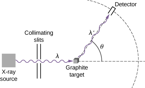
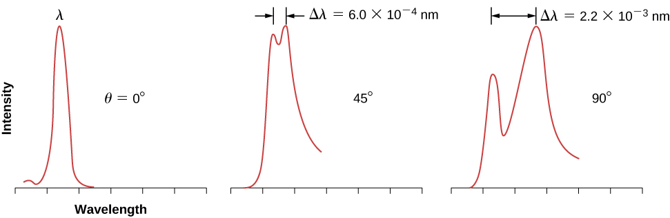
The schematics of Compton’s experimental setup are shown in [link] . The idea of the experiment is straightforward: Monochromatic X-rays with wavelength are incident on a sample of graphite (the “target”), where they interact with atoms inside the sample; they later emerge as scattered X-rays with wavelength A detector placed behind the target can measure the intensity of radiation scattered in any direction with respect to the direction of the incident X-ray beam. This scattering angle , is the angle between the direction of the scattered beam and the direction of the incident beam. In this experiment, we know the intensity and the wavelength of the incoming (incident) beam; and for a given scattering angle we measure the intensity and the wavelength of the outgoing (scattered) beam. Typical results of these measurements are shown in [link] , where the x -axis is the wavelength of the scattered X-rays and the y -axis is the intensity of the scattered X-rays, measured for different scattering angles (indicated on the graphs). For all scattering angles (except for we measure two intensity peaks. One peak is located at the wavelength which is the wavelength of the incident beam. The other peak is located at some other wavelength, The two peaks are separated by which depends on the scattering angle of the outgoing beam (in the direction of observation). The separation is called the Compton shift .
Notification Switch
Would you like to follow the 'University physics volume 3' conversation and receive update notifications?

|
|

|
|

|
|

|
|

|
|

|
|

|
|

|
|

|
|

|