

| << Chapter < Page | Chapter >> Page > |
In the preceding chapter, we saw that particles act in some cases like particles and in other cases like waves. But what does it mean for a particle to “act like a wave”? What precisely is “waving”? What rules govern how this wave changes and propagates? How is the wave function used to make predictions? For example, if the amplitude of an electron wave is given by a function of position and time, , defined for all x , where exactly is the electron? The purpose of this chapter is to answer these questions.
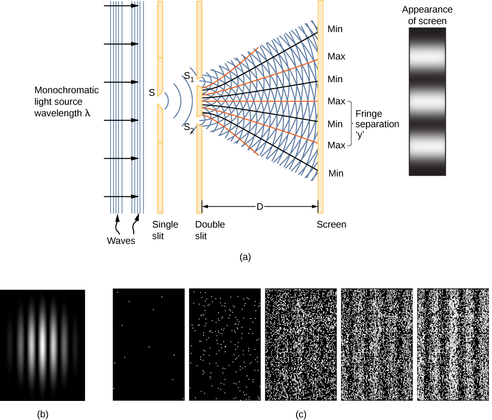
A clue to the physical meaning of the wave function is provided by the two-slit interference of monochromatic light ( [link] ). (See also Electromagnetic Waves and Interference .) The wave function of a light wave is given by E ( x , t ), and its energy density is given by , where E is the electric field strength. The energy of an individual photon depends only on the frequency of light, so is proportional to the number of photons. When light waves from interfere with light waves from at the viewing screen (a distance D away), an interference pattern is produced (part (a) of the figure). Bright fringes correspond to points of constructive interference of the light waves, and dark fringes correspond to points of destructive interference of the light waves (part (b)).
Suppose the screen is initially unexposed to light. If the screen is exposed to very weak light, the interference pattern appears gradually ( [link] (c), left to right). Individual photon hits on the screen appear as dots. The dot density is expected to be large at locations where the interference pattern will be, ultimately, the most intense. In other words, the probability (per unit area) that a single photon will strike a particular spot on the screen is proportional to the square of the total electric field, at that point. Under the right conditions, the same interference pattern develops for matter particles, such as electrons.
Visit this interactive simulation to learn more about quantum wave interference.
The square of the matter wave in one dimension has a similar interpretation as the square of the electric field . It gives the probability that a particle will be found at a particular position and time per unit length, also called the probability density . The probability ( P ) a particle is found in a narrow interval ( x , x + dx ) at time t is therefore
(Later, we define the magnitude squared for the general case of a function with “imaginary parts.”) This probabilistic interpretation of the wave function is called the Born interpretation . Examples of wave functions and their squares for a particular time t are given in [link] .
Notification Switch
Would you like to follow the 'University physics volume 3' conversation and receive update notifications?

|
|

|
|

|
|

|
|

|
|

|
|

|
|

|
|
|
|
|

|