

| << Chapter < Page | Chapter >> Page > |
Magnetic flux depends on three factors: the strength of the magnetic field, the area through which the field lines pass, and the orientation of the field with the surface area. If any of these quantities varies, a corresponding variation in magnetic flux occurs. So far, we’ve only considered flux changes due to a changing field. Now we look at another possibility: a changing area through which the field lines pass including a change in the orientation of the area.
Two examples of this type of flux change are represented in [link] . In part (a), the flux through the rectangular loop increases as it moves into the magnetic field, and in part (b), the flux through the rotating coil varies with the angle .
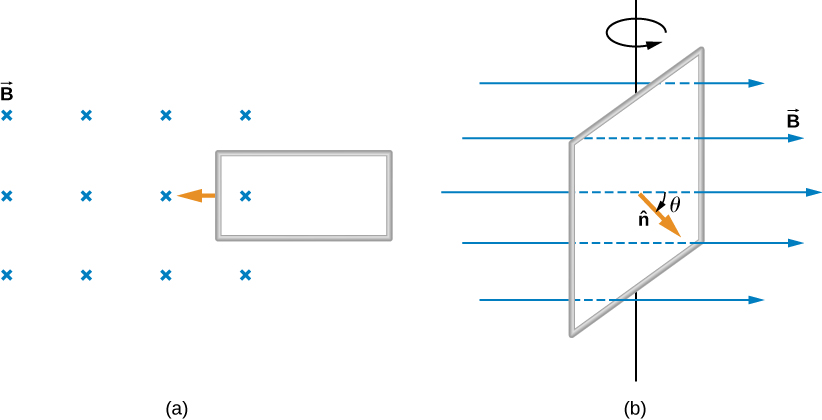
It’s interesting to note that what we perceive as the cause of a particular flux change actually depends on the frame of reference we choose. For example, if you are at rest relative to the moving coils of [link] , you would see the flux vary because of a changing magnetic field—in part (a), the field moves from left to right in your reference frame, and in part (b), the field is rotating. It is often possible to describe a flux change through a coil that is moving in one particular reference frame in terms of a changing magnetic field in a second frame, where the coil is stationary. However, reference-frame questions related to magnetic flux are beyond the level of this textbook. We’ll avoid such complexities by always working in a frame at rest relative to the laboratory and explain flux variations as due to either a changing field or a changing area.
Now let’s look at a conducting rod pulled in a circuit, changing magnetic flux. The area enclosed by the circuit ‘MNOP’ of [link] is lx and is perpendicular to the magnetic field, so we can simplify the integration of [link] into a multiplication of magnetic field and area. The magnetic flux through the open surface is therefore
Since B and l are constant and the velocity of the rod is we can now restate Faraday’s law, [link] , for the magnitude of the emf in terms of the moving conducting rod as
The current induced in the circuit is the emf divided by the resistance or
Furthermore, the direction of the induced emf satisfies Lenz’s law, as you can verify by inspection of the figure.
This calculation of motionally induced emf is not restricted to a rod moving on conducting rails. With as the starting point, it can be shown that holds for any change in flux caused by the motion of a conductor. We saw in Faraday’s Law that the emf induced by a time-varying magnetic field obeys this same relationship, which is Faraday’s law. Thus Faraday’s law holds for all flux changes , whether they are produced by a changing magnetic field, by motion, or by a combination of the two.
Notification Switch
Would you like to follow the 'University physics volume 2' conversation and receive update notifications?

|
|

|
|

|
|

|
|

|
|

|
|
|
|

|
|

|
|

|