

| << Chapter < Page | Chapter >> Page > |
Two of the most common and useful electromagnetic devices are called solenoids and toroids. In one form or another, they are part of numerous instruments, both large and small. In this section, we examine the magnetic field typical of these devices.
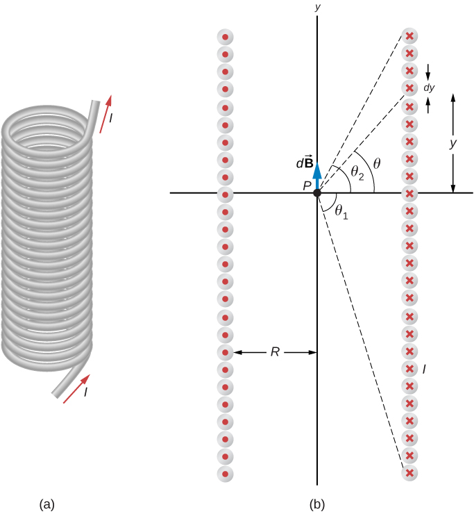
A long wire wound in the form of a helical coil is known as a solenoid . Solenoids are commonly used in experimental research requiring magnetic fields. A solenoid is generally easy to wind, and near its center, its magnetic field is quite uniform and directly proportional to the current in the wire.
[link] shows a solenoid consisting of N turns of wire tightly wound over a length L . A current I is flowing along the wire of the solenoid. The number of turns per unit length is N / L ; therefore, the number of turns in an infinitesimal length dy are ( N / L ) dy turns. This produces a current
We first calculate the magnetic field at the point P of [link] . This point is on the central axis of the solenoid. We are basically cutting the solenoid into thin slices that are dy thick and treating each as a current loop. Thus, dI is the current through each slice. The magnetic field due to the current dI in dy can be found with the help of [link] and [link] :
where we used [link] to replace dI . The resultant field at P is found by integrating along the entire length of the solenoid. It’s easiest to evaluate this integral by changing the independent variable from y to From inspection of [link] , we have:
Taking the differential of both sides of this equation, we obtain
When this is substituted into the equation for we have
which is the magnetic field along the central axis of a finite solenoid.
Of special interest is the infinitely long solenoid, for which From a practical point of view, the infinite solenoid is one whose length is much larger than its radius In this case, and Then from [link] , the magnetic field along the central axis of an infinite solenoid is
or
where n is the number of turns per unit length. You can find the direction of with a right-hand rule: Curl your fingers in the direction of the current, and your thumb points along the magnetic field in the interior of the solenoid.
We now use these properties, along with Ampère’s law, to calculate the magnitude of the magnetic field at any location inside the infinite solenoid. Consider the closed path of [link] . Along segment 1, is uniform and parallel to the path. Along segments 2 and 4, is perpendicular to part of the path and vanishes over the rest of it. Therefore, segments 2 and 4 do not contribute to the line integral in Ampère’s law. Along segment 3, because the magnetic field is zero outside the solenoid. If you consider an Ampère’s law loop outside of the solenoid, the current flows in opposite directions on different segments of wire. Therefore, there is no enclosed current and no magnetic field according to Ampère’s law. Thus, there is no contribution to the line integral from segment 3. As a result, we find
Notification Switch
Would you like to follow the 'University physics volume 2' conversation and receive update notifications?

|
|

|
|

|
|

|
|

|
|

|
|

|
|

|
|

|
|

|