<< Chapter < Page Chapter >> Page >

In unit vector notation, the position vectors are

r ( t 1 ) = 6770. km j ^ r ( t 2 ) = 6770. km ( cos 45 ° ) i ^ + 6770. km ( sin ( −45 ° ) ) j ^ .

Evaluating the sine and cosine, we have

r ( t 1 ) = 6770. j ^ r ( t 2 ) = 4787 i ^ 4787 j ^ .

Now we can find Δ r , the displacement of the satellite:

Δ r = r ( t 2 ) r ( t 1 ) = 4787 i ^ 11,557 j ^ .

The magnitude of the displacement is | Δ r | = ( 4787 ) 2 + ( −11,557 ) 2 = 12,509 km . The angle the displacement makes with the x- axis is θ = tan −1 ( −11,557 4787 ) = −67.5 ° .

Significance

Plotting the displacement gives information and meaning to the unit vector solution to the problem. When plotting the displacement, we need to include its components as well as its magnitude and the angle it makes with a chosen axis—in this case, the x -axis ( [link] ).

An x y coordinate system is shown. Positive x is to the east and positive y to the north. Vector delta r sub x points east and has magnitude 4797 kilometers. Vector delta r sub y points south and has magnitude 11,557 kilometers. Vector delta r points to the southeast, starting at the tail of delta r sub x and ending at the head of delta r sub y and has magnitude 12,509 kilometers.
Displacement vector with components, angle, and magnitude.

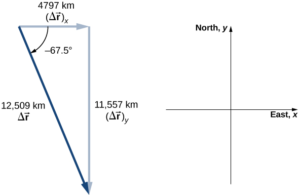
Note that the satellite took a curved path along its circular orbit to get from its initial position to its final position in this example. It also could have traveled 4787 km east, then 11,557 km south to arrive at the same location. Both of these paths are longer than the length of the displacement vector. In fact, the displacement vector gives the shortest path between two points in one, two, or three dimensions.

Many applications in physics can have a series of displacements, as discussed in the previous chapter. The total displacement is the sum of the individual displacements, only this time, we need to be careful, because we are adding vectors. We illustrate this concept with an example of Brownian motion.

Brownian motion

Brownian motion is a chaotic random motion of particles suspended in a fluid, resulting from collisions with the molecules of the fluid. This motion is three-dimensional. The displacements in numerical order of a particle undergoing Brownian motion could look like the following, in micrometers ( [link] ):

Δ r 1 = 2.0 i ^ + j ^ + 3.0 k ^ Δ r 2 = i ^ + 3.0 k ^ Δ r 3 = 4.0 i ^ 2.0 j ^ + k ^ Δ r 4 = −3.0 i ^ + j ^ + 2.0 k ^ .

What is the total displacement of the particle from the origin?

An x y z coordinate system with distances measured in micrometers and ranging from -10 to +10 micrometers is shown. The displacements delta r sub 1 equals 2 I hat plus j hat plus 2 k hat, delta r sub 2 equals -1 I hat plus 3 k hat, and delta r sub 3 equals -3 I hat plus j hat plus 2 k hat are shown as blue line segments. Vector r 1 hat starts at the origin. Each subsequent displacement starts where the previous one ends. Vector delta r total is shown as a red line starting at the origin and ending at the end of vector delta r 4. Delta r total equals 2 I hat plus 0 y hat plus 9 k hat.
Trajectory of a particle undergoing random displacements of Brownian motion. The total displacement is shown in red.

Solution

We form the sum of the displacements and add them as vectors:

Δ r Total = Δ r i = Δ r 1 + Δ r 2 + Δ r 3 + Δ r 4 = ( 2.0 1.0 + 4.0 3.0 ) i ^ + ( 1.0 + 0 2.0 + 1.0 ) j ^ + ( 3.0 + 3.0 + 1.0 + 2.0 ) k ^ = 2.0 i ^ + 0 j ^ + 9.0 k ^ μ m .

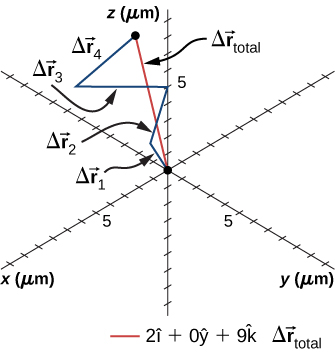
To complete the solution, we express the displacement as a magnitude and direction,

| Δ r Total | = 2.0 2 + 0 2 + 9.0 2 = 9.2 μ m, θ = tan −1 ( 9 2 ) = 77 ° ,

with respect to the x -axis in the xz- plane.

Significance

From the figure we can see the magnitude of the total displacement is less than the sum of the magnitudes of the individual displacements.

Got questions? Get instant answers now!

Velocity vector

In the previous chapter we found the instantaneous velocity by calculating the derivative of the position function with respect to time. We can do the same operation in two and three dimensions, but we use vectors. The instantaneous velocity vector    is now

v ( t ) = lim Δ t 0 r ( t + Δ t ) r ( t ) Δ t = d r d t .

Let’s look at the relative orientation of the position vector and velocity vector graphically. In [link] we show the vectors r ( t ) and r ( t + Δ t ) , which give the position of a particle moving along a path represented by the gray line. As Δ t goes to zero, the velocity vector, given by [link] , becomes tangent to the path of the particle at time t .

Practice Key Terms 3

Get Jobilize Job Search Mobile App in your pocket Now!

Get it on Google Play Download on the App Store Now


Source:  OpenStax, University physics volume 1. OpenStax CNX. Sep 19, 2016 Download for free at http://cnx.org/content/col12031/1.5
Google Play and the Google Play logo are trademarks of Google Inc.

Notification Switch

Would you like to follow the 'University physics volume 1' conversation and receive update notifications?

Ask