<< Chapter < Page Chapter >> Page >

Equations of shm

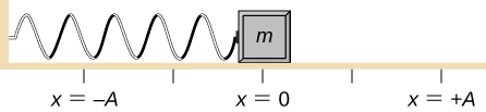
Consider a block attached to a spring on a frictionless table ( [link] ). The equilibrium position    (the position where the spring is neither stretched nor compressed) is marked as x = 0 . At the equilibrium position, the net force is zero.

A block is attached to a horizontal spring and placed on a frictionless table. The equilibrium position, where the spring is neither extended nor compressed, is marked as x=0. A position to the left of the block is marked as x = - A and a position the same distance to the right of the block is marked as x = + A.
A block is attached to a spring and placed on a frictionless table. The equilibrium position, where the spring is neither extended nor compressed, is marked as x = 0 .

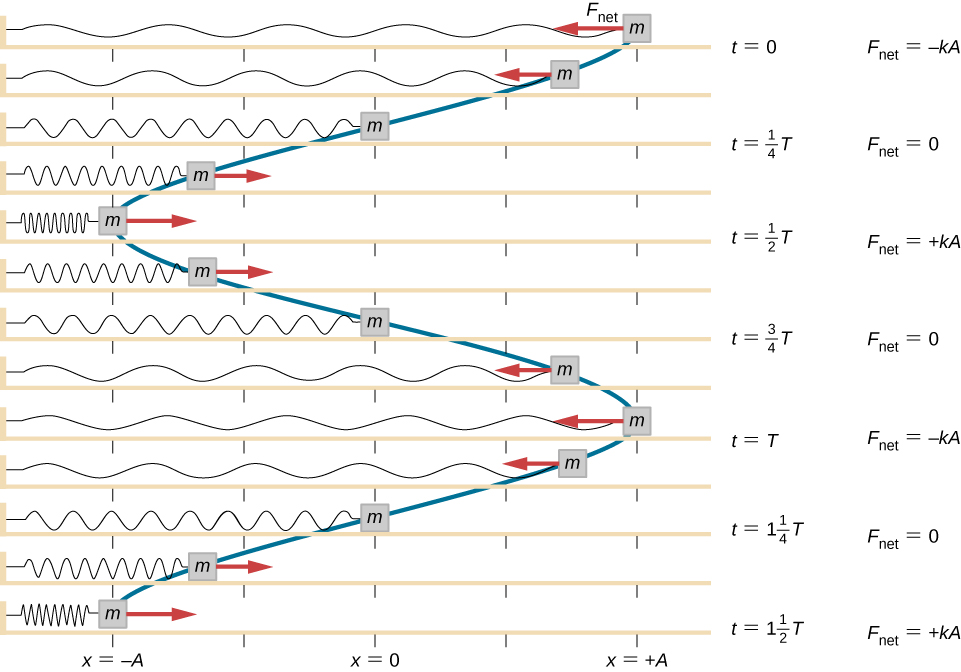
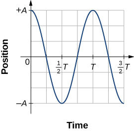
Work is done on the block to pull it out to a position of x = + A , and it is then released from rest. The maximum x -position ( A ) is called the amplitude of the motion. The block begins to oscillate in SHM between x = + A and x = A , where A is the amplitude of the motion and T is the period of the oscillation. The period is the time for one oscillation. [link] shows the motion of the block as it completes one and a half oscillations after release. [link] shows a plot of the position of the block versus time. When the position is plotted versus time, it is clear that the data can be modeled by a cosine function with an amplitude A and a period T . The cosine function cos θ repeats every multiple of 2 π , whereas the motion of the block repeats every period T . However, the function cos ( 2 π T t ) repeats every integer multiple of the period. The maximum of the cosine function is one, so it is necessary to multiply the cosine function by the amplitude A .

x ( t ) = A cos ( 2 π T t ) = A cos ( ω t ) .

Recall from the chapter on rotation that the angular frequency equals ω = d θ d t . In this case, the period is constant, so the angular frequency is defined as 2 π divided by the period, ω = 2 π T .

A series of illustrations of a mass, attached to a horizontal spring and sliding on a horizontal surface, is shown. The position of the mass, the spring, and the force on the mass are illustrated every eighth period from t = 0 to t = one and a half periods. The illustrations are aligned vertically and the positions of the mass are connected from one graph to the next using a blue line, creating a graph of the position (horizontal) dependence on time (vertical). The x = 0 position is at the center of the horizontal surface. In the top graph, the mass is at x = +A, the net force is to the left and is equal to – k A. The spring is stretched the maximum amount. The time is t = 0. In the second graph, the mass is between x = +A/2 and x = A, the net force is to the left and smaller than in the previous graph. The spring is stretched less than at t=0. In the third graph, the mass is at x = 0, there is no net force. The spring is relaxed. The time is t = one quarter T. In the fourth graph, the mass is between x = -A/2 and x = -A, the net force is to the right. The magnitude of the force is the same as that in the second graph. The spring is somewhat compressed. In the fifth graph, the mass is at x = -A, the net force is to the right and is equal to + k A. The spring is compressed the maximum amount. The time is t = 1/2 T. In the sixth graph, the mass is between x = -A/2 and x = -A, the net force is to the right. The magnitude of the force is the same as that in the second graph. The spring is somewhat compressed. This graph is identical to the fourth graph. In the seventh graph, the mass is at x = 0, there is no net force. The spring is relaxed. The time is t = 3/4 T. This graph is identical to the third graph. In the eighth graph, the mass is between x = +A/2 and x = A, the net force is to the left. This graph is identical to the second graph. In the ninth graph, the mass is at x = +A, the net force is to the left and is equal to – k A. The spring is stretched the maximum amount. The time is t = 0. This graph is identical to the first (top) graph. The remaining four graphs repeat the second, third, fourth and fifth graphs, with the eleventh graph’s time at t = 1 and 1/4 T and the thirteenth at t = 1 and 1/2 T. The curve connecting the positions of the mass forms a vertical sinusoidal curve.
A block is attached to one end of a spring and placed on a frictionless table. The other end of the spring is anchored to the wall. The equilibrium position, where the net force equals zero, is marked as x = 0 m . Work is done on the block, pulling it out to x = + A , and the block is released from rest. The block oscillates between x = + A and x = A . The force is also shown as a vector.
A graph of the position on the vertical axis as a function of time on the horizontal axis. The vertical scale is from – A to +A and the horizontal scale is from 0 to 3/2 T. The curve is a cosine function, with a value of +A at time zero and again at time T.
A graph of the position of the block shown in [link] as a function of time. The position can be modeled as a periodic function, such as a cosine or sine function.

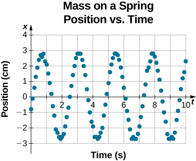
The equation for the position as a function of time x ( t ) = A cos ( ω t ) is good for modeling data, where the position of the block at the initial time t = 0.00 s is at the amplitude A and the initial velocity is zero. Often when taking experimental data, the position of the mass at the initial time t = 0.00 s is not equal to the amplitude and the initial velocity is not zero. Consider 10 seconds of data collected by a student in lab, shown in [link] .

Data of position versus time for a mass on a spring. The horizontal axis is time t in seconds, ranging from 0 to 10 seconds. The vertical axis is position x in centimeters, ranging from -3 centimeters to 4 centimeters. The data is shown as points and appears to be taken at regular intervals at about 10 points per second. The data oscillates sinusoidally, with a little over four full cycles during the 10 seconds of data shown. The position at t=0 is x = -0.8 centimeters. The position is at a maximum of x = 3 centimeters at about t = 0.6 s, 3.1 s, 5.5 s, and 7.9 s. The position is at the minimum of x = -3 centimeters at about t=1.9 s, 4.3 s, 6.7 s, and 9.0 s.
Data collected by a student in lab indicate the position of a block attached to a spring, measured with a sonic range finder. The data are collected starting at time t = 0.00 s, but the initial position is near position x 0.80 cm 3.00 cm , so the initial position does not equal the amplitude x 0 = + A . The velocity is the time derivative of the position, which is the slope at a point on the graph of position versus time. The velocity is not v = 0.00 m/s at time t = 0.00 s , as evident by the slope of the graph of position versus time, which is not zero at the initial time.

Get Jobilize Job Search Mobile App in your pocket Now!

Get it on Google Play Download on the App Store Now


Source:  OpenStax, University physics volume 1. OpenStax CNX. Sep 19, 2016 Download for free at http://cnx.org/content/col12031/1.5
Google Play and the Google Play logo are trademarks of Google Inc.

Notification Switch

Would you like to follow the 'University physics volume 1' conversation and receive update notifications?

Ask