<< Chapter < Page Chapter >> Page >

The angular frequency for damped harmonic motion becomes

ω = ω 0 2 ( b 2 m ) 2 .
The figure shows a graph of displacement, x in meters, along the vertical axis, versus time in seconds along the horizontal axis. The displacement ranges from minus A sub zero to plus A sub zero and the time ranges from 0 to 10 T. The displacement, shown by a blue curve, oscillates between positive maxima and negative minima, forming a wave whose amplitude is decreasing gradually as we move far from t=0. The time, T, between adjacent crests remains the same throughout. The envelope, the smooth curve that connects the crests and another smooth curve that connects the troughs of the oscillations, is shown as a pair of dashed red lines. The upper curve connecting the crests is labeled as plus A sub zero times e to the quantity minus b t over 2 m. The lower curve connecting the troughs is labeled as minus A sub zero times e to the quantity minus b t over 2 m.
Position versus time for the mass oscillating on a spring in a viscous fluid. Notice that the curve appears to be a cosine function inside an exponential envelope.

Recall that when we began this description of damped harmonic motion, we stated that the damping must be small. Two questions come to mind. Why must the damping be small? And how small is small? If you gradually increase the amount of damping in a system, the period and frequency begin to be affected, because damping opposes and hence slows the back and forth motion. (The net force is smaller in both directions.) If there is very large damping, the system does not even oscillate—it slowly moves toward equilibrium. The angular frequency is equal to

ω = k m ( b 2 m ) 2 .

As b increases, k m ( b 2 m ) 2 becomes smaller and eventually reaches zero when b = 4 m k . If b becomes any larger, k m ( b 2 m ) 2 becomes a negative number and k m ( b 2 m ) 2 is a complex number.

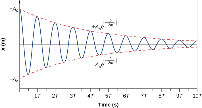
[link] shows the displacement of a harmonic oscillator for different amounts of damping. When the damping constant is small, b < 4 m k , the system oscillates while the amplitude of the motion decays exponentially. This system is said to be underdamped    , as in curve (a). Many systems are underdamped, and oscillate while the amplitude decreases exponentially, such as the mass oscillating on a spring. The damping may be quite small, but eventually the mass comes to rest. If the damping constant is b = 4 m k , the system is said to be critically damped    , as in curve (b). An example of a critically damped system is the shock absorbers in a car. It is advantageous to have the oscillations decay as fast as possible. Here, the system does not oscillate, but asymptotically approaches the equilibrium condition as quickly as possible. Curve (c) in [link] represents an overdamped    system where b > 4 m k . An overdamped system will approach equilibrium over a longer period of time.

The position, x in meters on the vertical axis, versus time in seconds on the horizontal axis, with varying degrees of damping. No scale is given for either axis. All three curves start at the same positive position at time zero. Blue curve a, labeled with b squared is less than 4 m k, undergoes a little over two and a quarter oscillations of decreasing amplitude and constant period. Red curve b, labeled with b squared is equal to 4 m k, decreases at t=0 less rapidly than the blue curve, but does not oscillate. The red curve approaches x=0 asymptotically, and is nearly zero within one oscillation of the blue curve. Green curve c, labeled with b squared is greater than 4 m k, decreases at t=0 less rapidly than the red curve, and does not oscillate. The green curve approaches x=0 asymptotically, but is still noticeably above zero at the end of the graph, after more than two oscillations of the blue curve.
The position versus time for three systems consisting of a mass and a spring in a viscous fluid. (a) If the damping is small ( b < 4 m k ) , the mass oscillates, slowly losing amplitude as the energy is dissipated by the non-conservative force(s). The limiting case is (b) where the damping is ( b = 4 m k ) . (c) If the damping is very large ( b > 4 m k ) , the mass does not oscillate when displaced, but attempts to return to the equilibrium position.

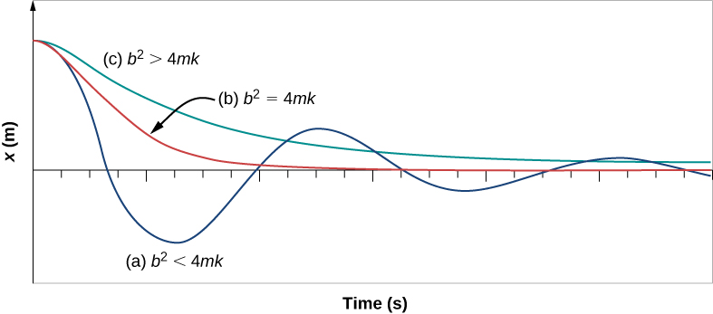
Critical damping is often desired, because such a system returns to equilibrium rapidly and remains at equilibrium as well. In addition, a constant force applied to a critically damped system moves the system to a new equilibrium position in the shortest time possible without overshooting or oscillating about the new position.

Check Your Understanding Why are completely undamped harmonic oscillators so rare?

Friction often comes into play whenever an object is moving. Friction causes damping in a harmonic oscillator.

Got questions? Get instant answers now!

Summary

  • Damped harmonic oscillators have non-conservative forces that dissipate their energy.
  • Critical damping returns the system to equilibrium as fast as possible without overshooting.
  • An underdamped system will oscillate through the equilibrium position.
  • An overdamped system moves more slowly toward equilibrium than one that is critically damped.

Conceptual questions

Give an example of a damped harmonic oscillator. (They are more common than undamped or simple harmonic oscillators.)

A car shock absorber.

Got questions? Get instant answers now!

How would a car bounce after a bump under each of these conditions?

(a) overdamping

(b) underdamping

(c) critical damping

Got questions? Get instant answers now!

Most harmonic oscillators are damped and, if undriven, eventually come to a stop. Why?

The second law of thermodynamics states that perpetual motion machines are impossible. Eventually the ordered motion of the system decreases and returns to equilibrium.

Got questions? Get instant answers now!

Problems

The amplitude of a lightly damped oscillator decreases by 3.0 % during each cycle. What percentage of the mechanical energy of the oscillator is lost in each cycle?

9%

Got questions? Get instant answers now!
Practice Key Terms 4

Get Jobilize Job Search Mobile App in your pocket Now!

Get it on Google Play Download on the App Store Now


Source:  OpenStax, University physics volume 1. OpenStax CNX. Sep 19, 2016 Download for free at http://cnx.org/content/col12031/1.5
Google Play and the Google Play logo are trademarks of Google Inc.

Notification Switch

Would you like to follow the 'University physics volume 1' conversation and receive update notifications?

Ask