

| << Chapter < Page | Chapter >> Page > |
Imagine a thin element of fluid at a depth h , as shown in [link] . Let the element have a cross-sectional area A and height . The forces acting upon the element are due to the pressures p ( y ) above and below it. The weight of the element itself is also shown in the free-body diagram.
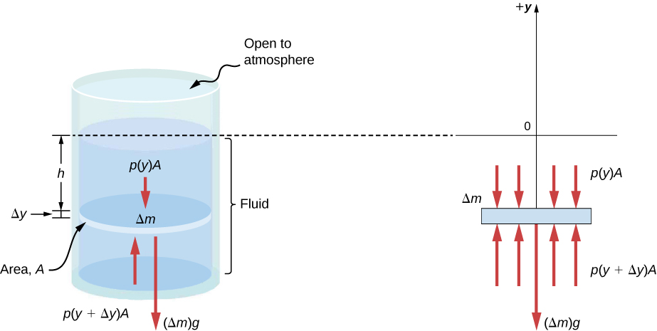
Since the element of fluid between y and is not accelerating, the forces are balanced. Using a Cartesian y -axis oriented up, we find the following equation for the y -component:
Note that if the element had a non-zero y -component of acceleration, the right-hand side would not be zero but would instead be the mass times the y -acceleration. The mass of the element can be written in terms of the density of the fluid and the volume of the elements:
Putting this expression for into [link] and then dividing both sides by , we find
Taking the limit of the infinitesimally thin element , we obtain the following differential equation, which gives the variation of pressure in a fluid:
This equation tells us that the rate of change of pressure in a fluid is proportional to the density of the fluid. The solution of this equation depends upon whether the density ρ is constant or changes with depth; that is, the function ρ ( y ).
If the range of the depth being analyzed is not too great, we can assume the density to be constant. But if the range of depth is large enough for the density to vary appreciably, such as in the case of the atmosphere, there is significant change in density with depth. In that case, we cannot use the approximation of a constant density.
Let’s use [link] to work out a formula for the pressure at a depth h from the surface in a tank of a liquid such as water, where the density of the liquid can be taken to be constant.
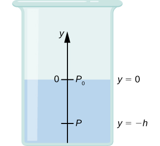
We need to integrate [link] from where the pressure is atmospheric pressure to the y -coordinate of the depth:
Hence, pressure at a depth of fluid on the surface of Earth is equal to the atmospheric pressure plus ρgh if the density of the fluid is constant over the height, as we found previously.
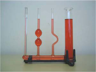
Note that the pressure in a fluid depends only on the depth from the surface and not on the shape of the container. Thus, in a container where a fluid can freely move in various parts, the liquid stays at the same level in every part, regardless of the shape, as shown in [link] .
The change in atmospheric pressure with height is of particular interest. Assuming the temperature of air to be constant, and that the ideal gas law of thermodynamics describes the atmosphere to a good approximation, we can find the variation of atmospheric pressure with height, when the temperature is constant. (We discuss the ideal gas law in a later chapter, but we assume you have some familiarity with it from high school and chemistry.) Let p ( y ) be the atmospheric pressure at height y . The density at y , the temperature T in the Kelvin scale (K), and the mass m of a molecule of air are related to the absolute pressure by the ideal gas law, in the form
Notification Switch
Would you like to follow the 'University physics volume 1' conversation and receive update notifications?

|
|

|
|

|
|

|
|

|
|

|
|
|
|
|

|
|
|
|
|

|