<< Chapter < Page Chapter >> Page >
a ( t ) = d d t v ( t ) .

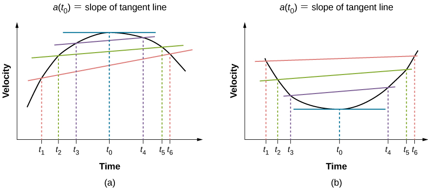
Thus, similar to velocity being the derivative of the position function, instantaneous acceleration is the derivative of the velocity function. We can show this graphically in the same way as instantaneous velocity. In [link] , instantaneous acceleration at time t 0 is the slope of the tangent line to the velocity-versus-time graph at time t 0 . We see that average acceleration a = Δ v Δ t approaches instantaneous acceleration as Δ t approaches zero. Also in part (a) of the figure, we see that velocity has a maximum when its slope is zero. This time corresponds to the zero of the acceleration function. In part (b), instantaneous acceleration at the minimum velocity is shown, which is also zero, since the slope of the curve is zero there, too. Thus, for a given velocity function, the zeros of the acceleration function give either the minimum or the maximum velocity.

Graph A shows velocity plotted versus time. Velocity increases from t1 to t2 and t3. It reaches maximum at t0. It decreases to t4 and continues to decrease to t5 and t6. The slope of the tangent line at t0 is indicated as the instantaneous velocity. Graph B shows velocity plotted versus time. Velocity decreases from t1 to t2 and t3. It reaches minimum at t0. It increases to t4 and continues to increase to t5 and t6. The slope of the tangent line at t0 is indicated as the instantaneous velocity.
In a graph of velocity versus time, instantaneous acceleration is the slope of the tangent line. (a) Shown is average acceleration a = Δ v Δ t = v f v i t f t i between times Δ t = t 6 t 1 , Δ t = t 5 t 2 , and Δ t = t 4 t 3 . When Δ t 0 , the average acceleration approaches instantaneous acceleration at time t 0. In view (a), instantaneous acceleration is shown for the point on the velocity curve at maximum velocity. At this point, instantaneous acceleration is the slope of the tangent line, which is zero. At any other time, the slope of the tangent line—and thus instantaneous acceleration—would not be zero. (b) Same as (a) but shown for instantaneous acceleration at minimum velocity.

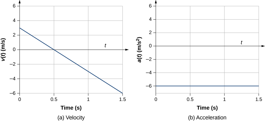
To illustrate this concept, let’s look at two examples. First, a simple example is shown using [link] (b), the velocity-versus-time graph of [link] , to find acceleration graphically. This graph is depicted in [link] (a), which is a straight line. The corresponding graph of acceleration versus time is found from the slope of velocity and is shown in [link] (b). In this example, the velocity function is a straight line with a constant slope, thus acceleration is a constant. In the next example, the velocity function is has a more complicated functional dependence on time.

Graph A shows velocity in meters per second plotted versus time in seconds. Graph is linear and has a negative constant slope. Graph B shows acceleration in meters per second square plotted versus time in seconds. Graph is linear and has a zero slope with the acceleration being equal to -6.
(a, b) The velocity-versus-time graph is linear and has a negative constant slope (a) that is equal to acceleration, shown in (b).

If we know the functional form of velocity, v ( t ), we can calculate instantaneous acceleration a ( t ) at any time point in the motion using [link] .

Calculating instantaneous acceleration

A particle is in motion and is accelerating. The functional form of the velocity is v ( t ) = 20 t 5 t 2 m/s .

  1. Find the functional form of the acceleration.
  2. Find the instantaneous velocity at t = 1, 2, 3, and 5 s.
  3. Find the instantaneous acceleration at t = 1, 2, 3, and 5 s.
  4. Interpret the results of (c) in terms of the directions of the acceleration and velocity vectors.

Strategy

We find the functional form of acceleration by taking the derivative of the velocity function. Then, we calculate the values of instantaneous velocity and acceleration from the given functions for each. For part (d), we need to compare the directions of velocity and acceleration at each time.

Practice Key Terms 2

Get Jobilize Job Search Mobile App in your pocket Now!

Get it on Google Play Download on the App Store Now


Source:  OpenStax, University physics volume 1. OpenStax CNX. Sep 19, 2016 Download for free at http://cnx.org/content/col12031/1.5
Google Play and the Google Play logo are trademarks of Google Inc.

Notification Switch

Would you like to follow the 'University physics volume 1' conversation and receive update notifications?

Ask