

| << Chapter < Page | Chapter >> Page > |
This can be simplified using the trigonometric identity
where and , giving us
which simplifies to
Notice that the resultant wave is a sine wave that is a function only of position, multiplied by a cosine function that is a function only of time. Graphs of y ( x , t ) as a function of x for various times are shown in [link] . The red wave moves in the negative x -direction, the blue wave moves in the positive x -direction, and the black wave is the sum of the two waves. As the red and blue waves move through each other, they move in and out of constructive interference and destructive interference.
Initially, at time the two waves are in phase, and the result is a wave that is twice the amplitude of the individual waves. The waves are also in phase at the time In fact, the waves are in phase at any integer multiple of half of a period:
At other times, the two waves are out of phase, and the resulting wave is equal to zero. This happens at
Notice that some x -positions of the resultant wave are always zero no matter what the phase relationship is. These positions are called node s . Where do the nodes occur? Consider the solution to the sum of the two waves
Finding the positions where the sine function equals zero provides the positions of the nodes.
There are also positions where y oscillates between . These are the antinode s . We can find them by considering which values of x result in .
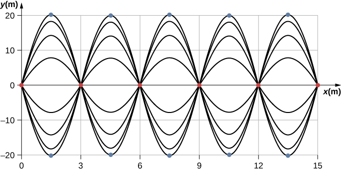
What results is a standing wave as shown in [link] , which shows snapshots of the resulting wave of two identical waves moving in opposite directions. The resulting wave appears to be a sine wave with nodes at integer multiples of half wavelengths. The antinodes oscillate between due to the cosine term, , which oscillates between .
The resultant wave appears to be standing still, with no apparent movement in the x -direction, although it is composed of one wave function moving in the positive, whereas the second wave is moving in the negative x -direction. [link] shows various snapshots of the resulting wave. The nodes are marked with red dots while the antinodes are marked with blue dots.
A common example of standing waves are the waves produced by stringed musical instruments. When the string is plucked, pulses travel along the string in opposite directions. The ends of the strings are fixed in place, so nodes appear at the ends of the strings—the boundary conditions of the system, regulating the resonant frequencies in the strings. The resonance produced on a string instrument can be modeled in a physics lab using the apparatus shown in [link] .
Notification Switch
Would you like to follow the 'University physics volume 1' conversation and receive update notifications?

|
|

|
|

|
|
|
|

|
|

|
|

|
|

|
|

|
|

|