Transform methods (Page 4/5)

Applied probability Page 4 / 5

This could, of course, have been achieved by using icalc and csort, which has the advantage that other functions of X and Y may be handled. Also, since the random variables are nonnegative, integer-valued, the MATLAB convolution function may beused (see [link] ). By repeated use of the function mgsum, we may obtain the distribution for the sum of more than two simple random variables. Them-functions mgsum3 and mgsum4 utilize this strategy.

The techniques for simple random variables may be used with the simple approximations to absolutely continuous random variables.

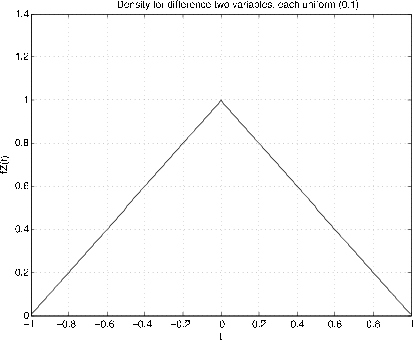
Difference of uniform distribution

The moment generating functions for the uniform and the symmetric triangular show that the latter appears naturally as the difference of two uniformly distributed randomvariables. We consider X and Y iid, uniform on [0,1].

tappr
Enter matrix [a b]of x-range endpoints  [0 1]
Enter number of x approximation points  200Enter density as a function of t  t<=1
Use row matrices X and PX as in the simple case[Z,PZ] = mgsum(X,-X,PX,PX);plot(Z,PZ/d)               % Divide by d to recover f(t)
%  plotting details   ---  see
[link]

Figure one is a density graph. It is titled, Density for difference two variables, each uniform (0, 1). The horizontal axis of the graph is labeled, t, and the vertical graph is labeled fZ(t). The plot of the density is triangular, beginning at (-1, 0), and increasing at a constant slope to point (0, 1). The graph continues after this point downward with a constant negative slope to point (1, 0). — Density for the difference of an independent pair, uniform (0,1).

Got questions? Get instant answers now!

The generating function

The form of the generating function for a nonnegative, integer-valued random variable exhibits a number of important properties.

X = \sum_{k = 0}^{\infty} k I_{A_{i}} (canonical form) p_{k} = P (A_{k}) = P (X = k) g_{X} (s) = \sum_{k = 0}^{\infty} s^{k} p_{k}

As a power series in s with nonnegative coefficients whose partial sums converge to one, the series converges at least for $| s | \leq 1$ .
The coefficients of the power series display the distribution: for value k the probability $p_{k} = P (X = k)$ is the coefficient of s ^k .
The power series expansion about the origin of an analytic function is unique. If the generating function is known in closed form, the unique power series expansionabout the origin determines the distribution. If the power series converges to a known closed form, that form characterizes the distribution,
For a simple random variable (i.e., $p_{k} = 0$ for $k > n$ ), g _X is a polynomial.

The poisson distribution

In [link] , above, we establish the generating function for $X \sim$ Poisson $(μ)$ from the distribution. Suppose, however, we simply encounter the generating function

g_{X} (s) = e^{m (s - 1)} = e^{- m} e^{m s}

From the known power series for the exponential, we get

g_{X} (s) = e^{- m} \sum_{k = 0}^{\infty} \frac{{(m s)}^{k}}{k!} = e^{- m} \sum_{k = 0}^{\infty} s^{k} \frac{m^{k}}{k!}

We conclude that

P (X = k) = e^{- m} \frac{m^{k}}{k!}, 0 \leq k

which is the Poisson distribution with parameter $μ = m$ .

Got questions? Get instant answers now!

For simple, nonnegative, integer-valued random variables, the generating functions are polynomials. Because of the product rule (T2) , the problem of determining the distribution for the sum of independentrandom variables may be handled by the process of multiplying polynomials. This may be done quickly and easily with the MATLAB convolution function.

Sum of independent simple random variables

Suppose the pair ${X, Y}$ is independent, with

g_{X} (s) = \frac{1}{10} (2 + 3 s + 3 s^{2} + 2 s^{5}) g_{Y} (s) = \frac{1}{10} (2 s + 4 s^{2} + 4 s^{3})

In the MATLAB function convolution, all powers of s must be accounted for by including zeros for the missing powers.

gx = 0.1*[2 3 3 0 0 2];      % Zeros for missing powers 3, 4gy = 0.1*[0 2 4 4];          % Zero  for missing power 0gz = conv(gx,gy);
a = ['       Z         PZ'];
b = [0:8;gz]';
disp(a)Z         PZ          % Distribution for Z = X + Y
disp(b)0         0
    1.0000    0.04002.0000    0.1400
    3.0000    0.26004.0000    0.2400
    5.0000    0.12006.0000    0.0400
    7.0000    0.08008.0000    0.0800

If mgsum were used, it would not be necessary to be concerned about missing powers and the corresponding zero coefficients.

Got questions? Get instant answers now!

<< Chapter < Page Page > Chapter >>

Read also:

Get Jobilize Job Search Mobile App in your pocket Now!

100% Free Mobile Applications
Receive real-time job alerts and never miss the right job again

Source: OpenStax, Applied probability. OpenStax CNX. Aug 31, 2009 Download for free at http://cnx.org/content/col10708/1.6

Google Play and the Google Play logo are trademarks of Google Inc.

Notification Switch

Would you like to follow the 'Applied probability' conversation and receive update notifications?

Ask

	Worldport Outside By Rachel Carlisle Start Quiz
	Macroeconomics MCQ By Candice Butts Start Quiz
	Anthropology Aesthetics Culture By Richley Crapo Start Assignment
©flickr: Miguel	Protozoal and Parasitic Infections By Cath Yu Start Quiz
	Real Estate Finance Exam 2003 By Tod McGrath Start Exam
	English Proficiency Test By Anindyo Mukhopadhyay Start Quiz
	Tournament Director Quiz By Eddie Unverzagt Start Quiz
	Western Political Thought MCQ By Saylor Foundation Start Quiz
	Socialism Command Economy By Robert Murphy Start Test
	Anthropology Religion Culture By Richley Crapo Start Assignment