<< Chapter < Page Chapter >> Page >
Transform coding is described and an analysis is performed for the simple 2-dimensional case, including a comparison to PCM.
  • In transform coding (TC), blocks of N input samples are transformed to N transform coefficients which are then quantized and transmitted. At the decoder, an inverse transformis applied to the quantized coefficients, yielding a reconstruction of the original waveform.By designing individual quantizers in accordance with the statistics of their inputs, it is possible to allocatebits in a more optimal manner, e.g., encoding the “more important” coefficients at a higher bit rate.
    This figure is a flowchart. Beginning on the left is an arrow labeled, x_0, ..., x_(n-1), pointing to the right at a large box labeled N x N transform. To the right of this large box are a series of short arrows pointing to the right labeled from top to bottom y_0, y_2, ..., y_(N-1). to the right of each of these arrows is a box labeled with a capital Q. To the right of each of the Q-boxes is another arrow labeled ytilde_0, ytilde_1, ..., ytilde_(N-1). At this point in the graph there is a large separation, as if the preceding arrows do not point at anything directly. To the left of the separation are a series of identical ytilde arrows, all pointing at a single large box labeled Inverse Transform. To the right of the large box is a final arrow pointing to the right labeled xtilde_0, ..., xtilde_(N-1). This figure is a flowchart. Beginning on the left is an arrow labeled, x_0, ..., x_(n-1), pointing to the right at a large box labeled N x N transform. To the right of this large box are a series of short arrows pointing to the right labeled from top to bottom y_0, y_2, ..., y_(N-1). to the right of each of these arrows is a box labeled with a capital Q. To the right of each of the Q-boxes is another arrow labeled ytilde_0, ytilde_1, ..., ytilde_(N-1). At this point in the graph there is a large separation, as if the preceding arrows do not point at anything directly. To the left of the separation are a series of identical ytilde arrows, all pointing at a single large box labeled Inverse Transform. To the right of the large box is a final arrow pointing to the right labeled xtilde_0, ..., xtilde_(N-1).
    N × N Transform Coder/Decoder with Scalar Quantization
  • Orthogonal Transforms:   From our perspective, an N × N “transform” will be any real-valued linear operation taking N input samples to N output samples, or transform coefficients.This operation can always be written in matrix form
    y ( m ) = T x ( m ) , T R N × N
    where x ( m ) and y ( m ) are vectors representing N × 1 blocks of input/output elements:
    x ( m ) = x ( m N ) , x ( m N - 1 ) , , x ( m N - N + 1 ) t y ( m ) = y ( m N ) , y ( m N - 1 ) , , y ( m N - N + 1 ) t .
    Intuition comes from considering the transform's basis vectors { t k } defined by the rows of the matrix
    T = --- t 0 t --- --- t 1 t --- -- t N - 1 t --
    since the coefficient y k = t k t x can be thought of as the result of a“comparison” between the k t h basis vector and the input x . These comparisons are defined by the inner product < t k , x > = t k t x which has a geometrical interpretation involving the angle θ k between vectors t k and x .
    < t k , x > = cos ( θ k ) t k 2 x 2 .
    When the vectors { t k } are mutually orthogonal, i.e., t k t t = 0 for k , the transform coefficients represent separate, unrelated features of the input.This property is convenient if the transform coefficients are independently quantized, as is typical in TC schemes.

    2 × 2 Transform coder

    Say that stationary zero-mean Gaussian source x ( m ) has autocorrelation r x ( 0 ) = 1 , r x ( 1 ) = ρ , and r x ( k ) = 0 for k > 1 . For a bit rate of R bits per sample, uniformly-quantized PCM implies a mean-squared reconstruction error of

    σ r 2 | PCM = Δ 2 12 | Δ = 2 x max / L L = 2 R = 1 3 x max 2 σ x 2 γ x σ x 2 2 - 2 R = γ x σ x 2 2 - 2 R .

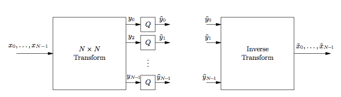
    For transform coding, say we choose linear transform

    T = t 0 t t 1 t = 1 2 1 1 1 - 1

    Setting x ( m ) = x ( 2 m ) x ( 2 m - 1 ) t and y ( m ) = Tx ( m ) , we find that the transformed coefficients have variance

    σ y 0 2 = E { | t 0 t x ( m ) | 2 } = 1 2 E | x ( 2 m ) + x ( 2 m - 1 ) | 2 = 1 2 2 r x ( 0 ) + 2 r x ( 1 ) = 1 + ρ
    σ y 1 2 = E { | t 1 t x ( m ) | 2 } = 1 2 E | x ( 2 m ) - x ( 2 m - 1 ) | 2 = 1 2 2 r x ( 0 ) - 2 r x ( 1 ) = 1 - ρ

    and using uniformly-quantized PCM on each coefficient we get mean-squared reconstruction errors

    σ q 0 2 = ( 1 + ρ ) γ x 2 - 2 R 0
    σ q 1 2 = ( 1 - ρ ) γ x 2 - 2 R 1 .

    We use the same quantizer performance factor γ x as before since linear operations preserve Gaussianity.
    For orthogonal matrices T , i.e., T - 1 = T t , we can show that the mean-squared reconstruction error σ r 2 equals the mean-squared quantization error:

    σ r 2 : = 1 N k = 0 N - 1 E x ˜ ( N m - k ) - x ( N m - k ) 2 ( here N = 2 ) = 1 N E x ˜ ( m ) - x ( m ) 2 = 1 N E T - 1 y ˜ ( m ) - x ( m ) 2 = 1 N E T - 1 y ( m ) + q ( m ) - x ( m ) 2 = 1 N E T - 1 Tx ( m ) + T - 1 q ( m ) - x ( m ) 2 = 1 N E T - 1 q ( m ) 2 = 1 N E q t ( m ) ( T - 1 ) t T - 1 I q ( m ) = 1 N E q ( m ) 2 = 1 N k = 0 N - 1 σ q k 2 .

    Since our 2 × 2 matrix is indeed orthogonal, we have mean-squared reconstruction error
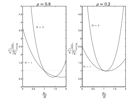
    σ r 2 | TC = 1 2 ( 1 + ρ ) γ x 2 - 2 R 0 + ( 1 - ρ ) γ x 2 - 2 R 1

    at bit rate of R 0 + R 1 bits per two samples. Comparing TC to PCM at equal bit rates (i.e. R 0 + R 1 = 2 R ),

    σ r 2 | TC σ r 2 | PCM = 1 2 ( 1 + ρ ) γ x 2 - 2 R 0 + ( 1 - ρ ) γ x 2 - 2 ( 2 R - R 0 ) γ x 2 - 2 R = ( 1 + ρ ) 2 2 ( R - R 0 ) - 1 + ( 1 - ρ ) 2 2 ( R 0 - R ) - 1 .

    [link] shows that (i) allocating a higher bit rate to the quantizer with stronger input signal can reduce the average reconstruction errorrelative to PCM, and (ii) the gain over PCM is higher when the input signal exhibits stronger correlation ρ . Also note that when R 0 = R 1 = R , there is no gain over PCM—a verification of the fact that σ r 2 = σ q 2 when T is orthogonal.

    This figure is composed of two cartesian graphs. Both graphs plot a horizontal axis, R_0/R, and a vertical axis, (σ^2_τ|TC)/(σ^2_τ|PCM). The vertical values range from 0 to 5, and the horizontal values range from 0 to 2. The graph on the left is titled ρ=0.8, and the graph on the right is labeled ρ=0.2. There are two curves on each graph, both parabolic in shape. On the ρ=0.8 graph, a curve labeled R=1 enters the page at (0, 3.5) and continues downward to a vertex at (1.75, 0.5). A sharper parabola labeled R=2 enters the graph at (0.4, 5) with a sharp downward slope to a vertex at (1.5, 0.5), where it then curves sharply upward and terminates at approximately (2, 1.6). On the ρ=0.2 graph, the R=1 curve enters at (0, 2.5) with a shallow downward slope  to a vertex at approximately (1.25, 1). A second curve, R=2, begins at (0.25, 5) with a strong downward slope to a vertex at approximately (1.1, 1), where it then continues upward to terminate at (1.9, 5). This figure is composed of two cartesian graphs. Both graphs plot a horizontal axis, R_0/R, and a vertical axis, (σ^2_τ|TC)/(σ^2_τ|PCM). The vertical values range from 0 to 5, and the horizontal values range from 0 to 2. The graph on the left is titled ρ=0.8, and the graph on the right is labeled ρ=0.2. There are two curves on each graph, both parabolic in shape. On the ρ=0.8 graph, a curve labeled R=1 enters the page at (0, 3.5) and continues downward to a vertex at (1.75, 0.5). A sharper parabola labeled R=2 enters the graph at (0.4, 5) with a sharp downward slope to a vertex at (1.5, 0.5), where it then curves sharply upward and terminates at approximately (2, 1.6). On the ρ=0.2 graph, the R=1 curve enters at (0, 2.5) with a shallow downward slope  to a vertex at approximately (1.25, 1). A second curve, R=2, begins at (0.25, 5) with a strong downward slope to a vertex at approximately (1.1, 1), where it then continues upward to terminate at (1.9, 5).
    Ratio of TC to PCM mean-squared reconstruction errors versus bit rate R 0 for two values of ρ .

Get Jobilize Job Search Mobile App in your pocket Now!

Get it on Google Play Download on the App Store Now


Source:  OpenStax, An introduction to source-coding: quantization, dpcm, transform coding, and sub-band coding. OpenStax CNX. Sep 25, 2009 Download for free at http://cnx.org/content/col11121/1.2
Google Play and the Google Play logo are trademarks of Google Inc.

Notification Switch

Would you like to follow the 'An introduction to source-coding: quantization, dpcm, transform coding, and sub-band coding' conversation and receive update notifications?

Ask