

| << Chapter < Page | Chapter >> Page > |
Linear predictive coding ( LPC ) is a popular technique for speech compression and speech synthesis.The theoretical foundations of both are described below.
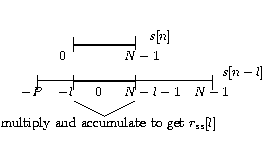
Correlation, a measure of similarity between two signals, is frequently used in the analysis of speech and other signals.The cross-correlation between two discrete-time signals and is defined as
Now consider the autocorrelation sequence , which describes the redundancy in the signal .
Another related method of measuring the redundancy in a signal is to compute its autocovariance
Linear prediction is a good tool for analysis of speech signals. Linear prediction models the human vocaltract as an infinite impulse response ( IIR ) system that produces the speech signal. For vowel sounds and other voiced regions of speech, whichhave a resonant structure and high degree of similarity over time shifts that are multiples of their pitch period, thismodeling produces an efficient representation of the sound. [link] shows how the resonant structure of a vowel could be captured by an IIR system.

The linear prediction problem can be stated as finding the coefficients which result in the best prediction (which minimizes mean-squared prediction error) of the speech sample in terms of the past samples , . The predicted sample is then given by Rabiner and Juang
Next we derive the frequency response of the system
in terms of the prediction coefficients
. In
[link] , when the predicted
sample equals the actual signal (
Initial Step: ,
for to .
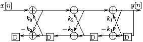
It is possible to use the prediction coefficients to synthesize the original sound by applying , the unit impulse, to the IIR system with lattice coefficients as shown in [link] . Applying to consecutive IIR systems (which represent consecutive speech segments) yields a longer segment of synthesizedspeech.
In this application, lattice filters are used rather than direct-form filters since the lattice filter coefficientshave magnitude less than one and, conveniently, are available directly as a result of the Levinson-Durbinalgorithm. If a direct-form implementation is desired instead, the coefficients must be factored into second-order stages with very small gains to yield a more stableimplementation.
When each segment of speech is synthesized in this manner,
two problems occur. First, the synthesized speech ismonotonous, containing no changes in pitch, because the
's, which represent pulses of air from the vocal
chords, occur with fixed periodicity equal to the analysissegment length; in normal speech, we vary the frequency of
air pulses from our vocal chords to change pitch. Second,the states of the lattice filter (
To estimate the pitch, we look at the autocorrelation coefficients of each segment. A large peak in the autocorrelation coefficient atlag implies the speech segment is periodic (or, more often, approximately periodic) with period . In synthesizing these segments, we recreate the periodicity by using an impulse train as input and varyingthe delay between impulses according to the pitch period. If the speech segment does not have a large peak in theautocorrelation coefficients, then the segment is an unvoiced signal which has no periodicity. Unvoiced segmentssuch as consonants are best reconstructed by using noise instead of an impulse train as input.
To reduce the discontinuity between segments, do not clear the states of the IIR model from one segment to the next.Instead, load the new set of reflection coefficients, , and continue with the lattice filter computation.
Notification Switch
Would you like to follow the 'Dsp laboratory with ti tms320c54x' conversation and receive update notifications?

|
|

|
|

|
|

|
|

|
|

|
|

|
|
|
|
|

|
|

|