

| << Chapter < Page | Chapter >> Page > |
A powerful data model for many applications is the geometric notion of a low-dimensional manifold . Data that possesses merely intrinsic degrees of freedom” can be assumed to lie on a -dimensional manifold in the high-dimensional ambient space. Once the manifold model is identified, any point on it can be representedusing essentially pieces of information. For instance, suppose a stationary camera of resolution observes a truck moving down along a straight line on a highway. Then, the set of images captured by the camera forms a 1-dimensional manifold in the image space . Another example is the set of images captured by a static camera observing a cube that rotates in 3 dimensions. ( [link] ).


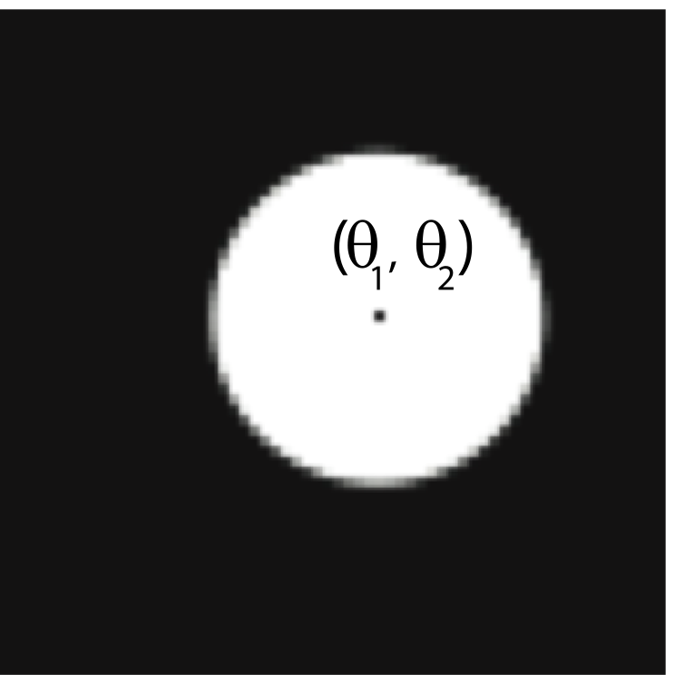
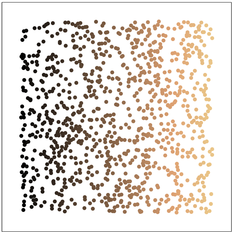
In many applications, it is beneficial to explicitly characterize the structure (alternately, identify the parameters) of the manifold formed by a set of observed signals. This is known as manifold learning and has been the subject of considerable study over the last several years; well-known manifold learning algorithms include Isomap [link] , LLE [link] , and Hessian eigenmaps [link] . An informal example is as follows: if a 2-dimensional manifold were to be imagined as the surface of a twisted sheet of rubber, manifold learning can be described as the process of “unraveling” the sheet and stretching it out on a 2D flat surface. [link] indicates the performance of Isomap on a simple 2-dimensional dataset comprising of images of a translating disk.

A linear, nonadaptive manifold dimensionality reduction technique has recently been introduced that employs the technique of random projections [link] . Consider a -dimensional manifold in the ambient space and its projection onto a random subspace of dimension ; note that . The result of [link] is that the pairwise metric structure of sample points from is preserved with high accuracy under projection from to . This is analogous to the result for compressive sensing of sparse signals (see "The restricted isometry property" ; however, the difference is that the number of projections required to preserve the ensemble structure does not depend on the sparsity of the individual images, but rather on the dimension of the underlying manifold.
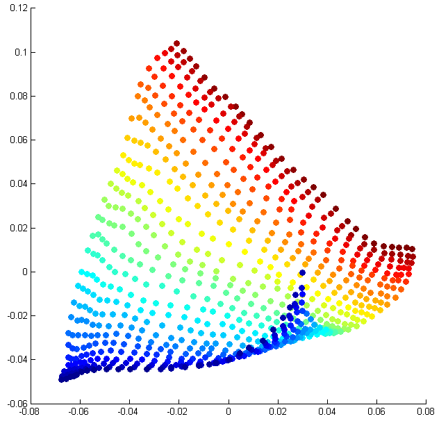
This result has far reaching implications; it suggests that a wide variety of signal processing tasks can be performed directly on the random projections acquired by these devices, thus saving valuable sensing, storage and processing costs. In particular, this enables provably efficient manifold learning in the projected domain [link] . [link] illustrates the performance of Isomap on the translating disk dataset under varying numbers of random projections.


The advantages of random projections extend even to cases where the original data is available in the ambient space . For example, consider a wireless network of cameras observing a static scene. The set of images captured by the cameras can be visualized as living on a low-dimensional manifold in the image space.To perform joint image analysis, the following steps might be executed:
In situations where is large and communication bandwidth is limited, the dominating costs will be in the firsttransmission/collation step. To reduce the communication expense, one may perform nonlinear image compression(such as JPEG) at each node before transmitting to the central processing. However, this requires a good deal of processing power ateach sensor, and the compression would have to be undone during the learning step, thus adding to overall computational costs.
As an alternative, every camera could encode its image by computing (either directly or indirectly) a small number of random projections tocommunicate to the central processor [link] . These random projections are obtained by linear operations on the data, and thus are cheaplycomputed. Clearly, in many situations it will be less expensive to store, transmit, and process such randomly projected versions of thesensed images. The method of random projections is thus a powerful tool for ensuring the stable embedding of low-dimensional manifolds into anintermediate space of reasonable size. It is now possible to think of settings involving a huge number of low-power devices that inexpensively capture, store, andtransmit a very small number of measurements of high-dimensional data.
Notification Switch
Would you like to follow the 'An introduction to compressive sensing' conversation and receive update notifications?

|
|

|
|

|
|

|
|

|
|
|
|

|
|

|
|

|
|

|