

| << Chapter < Page | Chapter >> Page > |
| Variable | Definition |
| Binary variables | |
| (ins | = 1 if individual has purchased supplementary insurance from any source |
| retire | = 1 if individual is retired |
| hstatusg | = 1 if individual assess his/her health status either as good, very good, or excellent |
| married | = 1 if married |
| hisp | = 1 if hispanic |
| female | = 1 if female |
| white | = 1 if white |
| sretire | = 1 if a retired spouse is present in household |
| Continuous variables | |
| age | Age of individual in years |
| hhincome | Household income |
| educyear | Years of education |
| chronic | Total number of chronic conditions |
| adl | Number of limitations on daily activity (up to 5) |
Stata commands
Place the data into the editor and then create a list of the independent variables. Now create a new variable equal to the log of income:
.generate linc = ln(hhinc)
[notice that 9 observations are eliminated.]
Create list of "extra" variables in order to shorten future commands:
. global extralist linc female white chronic adl sretire
Summarize the variables in order to check for obvious typos (output is suppressed):
.summarize ins retire $xlist $extralist
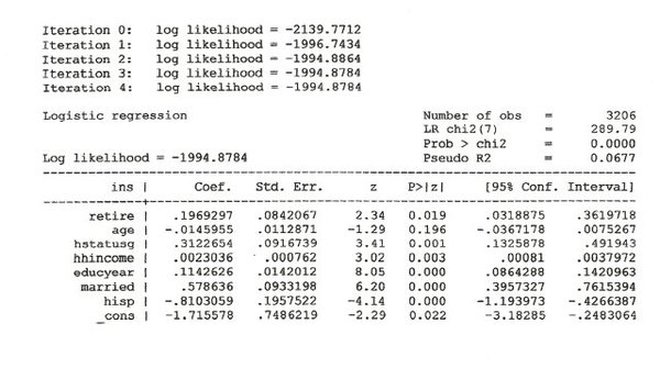
Estimate logit regression (output is shown in Figure 3):
.logit ins retire $xlist
Stata regression output.
Estimate and save results from several models (the Stata command "quietly" suppresses the output from the command):
. estimates store blogit
.quietly probit ins retire $xlist
.estimates store bprobit
.quietly regress ins retire $xlist
.estimates store bols
.quietly logit ins retire $list, vce(robust)
. estimates store blogitr
.quietly probit ins retire $xlist, vce(robust)
.estimates store bprobitr
.quietly regress ins retire $xlist, vce(robust)
.estimates store bolsr
We can create table for comparing the models (output is suppressed):
.estimates table blogit blogitr bprobit bprobitr bols bolsr, t stats(N ll) b(%8.4f) stfmt(%8.2f)
We now test for the presence of interaction variables:
.generate age2 = age*age
.generate agefem = age*fem
.generate agewhite = age*white
.generate agechronic = age*chronic
.global intlist age2 agefem agewhite agechronic
.quietly logit ins retire $xlist $intlist
.test $intlist
( 1) [ins]age2 = 0
( 2) [ins]agefem = 0
( 3) [ins]agewhite = 0
( 4) [ins]agechronic = 0
chi2( 4) = 7.45
Prob>chi2 = 0.1141
Likelihood ratio test
.quietly logit ins retire $xlist $intlist
.estimates store B
.quietly logit ins retire $xlist
.lrtest B
Likelihood-ratio test LR chi2(4) = 7.57
(Assumption: . nested in B) Prob>chi2 = 0.1088
Comparison with using the logistic command:
. logistic ins retire $xlist
The marginal effects at the mean will yield more useful results when the model is non-linear:
.quietly logit ins retire $xlist
.mfx
Let’s put the table comparing parameter estimates into a cleaned up table:
| Logit | Robust Logit | Probit | Robust Probit | OLS | Robust OLS | |
| Individual retired | 0.1969 | 0.1969 | 0.1184 | 0.1184 | 0.0409 | 0.0409 |
| (2.34) | (2.32) | (2.31) | (2.30) | (2.24) | (2.24) | |
| Age of individual | -0.0146 | -0.0146 | -0.0089 | -0.0089 | -0.0029 | -0.0029 |
| (-1.29) | (-1.29) | (-1.29) | (-1.32) | (-1.20) | (-1.25) | |
| Health status | 0.3123 | 0.3123 | 0.1977 | 0.1977 | 0.0656 | 0.0656 |
| (3.41) | (3.40) | (3.56) | (3.57) | (3.37) | (3.45) | |
| Household income | 0.0023 | 0.0023 | 0.0012 | 0.0012 | 0.0005 | 0.0005 |
| (3.02) | (2.01) | (3.19) | (2.21) | (3.58) | (2.63) | |
| Years of education | 0.1143 | 0.1143 | 0.0707 | 0.0707 | 0.0234 | 0.0234 |
| (8.05) | (7.96) | (8.34) | (8.33) | (8.15) | (8.63) | |
| Individual married | 0.5786 | 0.5786 | 0.3623 | 0.3623 | 0.1235 | 0.1235 |
| (6.20) | (6.15) | (6.47) | (6.16) | (6.38) | (6.62) | |
| Individual is an Hispanic | -0.8103 | -0.8103 | -0.4731 | -0.4731 | -0.1210 | -0.1210 |
| (-4.14) | (-4.18) | (-4.28) | (-4.36) | (-3.59) | (-4.49) | |
| Intercept | -1.7156 | -1.7156 | -1.0693 | -1.0693 | 0.1271 | 0.1271 |
| (-2.29) | (-2.36) | (-2.33) | (-2.40) | (0.79) | (0.83) | |
| Sample size | 3,206 | 3,206 | 3,206 | 3,206 | 3,206 | 3,206 |
| Log of the likelihood function | -1994.88 | -1994.88 | -1993.62 | -1993.62 | -2104.75 | -2104.75 |
Notification Switch
Would you like to follow the 'Econometrics for honors students' conversation and receive update notifications?

|
|

|
|

|
|

|
|
|
|
|

|
|

|
|

|
|

|
|

|