<< Chapter < Page Chapter >> Page >

Convolution and its numerical approximation

The output y ( t ) size 12{y \( t \) } {} of a continuous-time linear time-invariant (LTI) system is related to its input x ( t ) size 12{x \( t \) } {} and the system impulse response h ( t ) size 12{h \( t \) } {} through the convolution integral expressed as (for details on the theory of convolution and LTI systems, refer to signals and systems textbooks, for example, references [link] - [link] ):

y ( t ) = h ( t τ ) x ( τ ) size 12{y \( t \) = Int cSub { size 8{ - infinity } } cSup { size 8{ infinity } } {h \( t - τ \) x \( τ \) dτ} } {}

For a computer program to perform the above continuous-time convolution integral, a numerical approximation of the integral is needed noting that computer programs operate in a discrete – not continuous – fashion. One way to approximate the continuous functions in the Equation (1) integral is to use piecewise constant functions. Define δ Δ ( t ) size 12{δ rSub { size 8{Δ} } \( t \) } {} to be a rectangular pulse of width Δ size 12{Δ} {} and height 1, centered at t = 0 size 12{t=0} {} :

δ Δ ( t ) = { 1 Δ / 2 t Δ / 2 0 otherwise size 12{δ rSub { size 8{Δ} } \( t \) = left lbrace matrix { 1 {} # - Δ/2<= t<= Δ/2 {} ## 0 {} # ital "otherwise"{}} right none } {}

Approximate a continuous function x ( t ) size 12{x \( t \) } {} with a piecewise constant function x Δ ( t ) size 12{x rSub { size 8{Δ} } \( t \) } {} as a sequence of pulses spaced every Δ size 12{Δ} {} seconds in time with heights x ( ) size 12{x \( kΔ \) } {} :

x Δ ( t ) = k = x ( ) δ Δ ( t ) size 12{x rSub { size 8{Δ} } \( t \) = Sum cSub { size 8{k= - infinity } } cSup { size 8{ infinity } } {x \( kΔ \) δ rSub { size 8{Δ} } \( t - kΔ \) } } {}

It can be shown in the limit as Δ 0, x Δ ( t ) x ( t ) size 12{Δ rightarrow 0,x rSub { size 8{Δ} } \( t \) rightarrow x \( t \) } {} . As an example, 
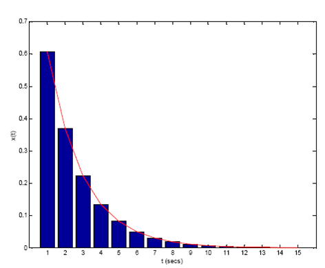
[link] shows the approximation of a decaying exponential x ( t ) = exp ( t 2 ) size 12{x \( t \) ="exp" \( - { {t} over {2} } \) } {} starting from 0 using Δ = 1 size 12{Δ=1} {} . Similarly, h ( t ) size 12{h \( t \) } {} can be approximated by

h Δ ( t ) = k = h ( ) δ Δ ( t ) size 12{h rSub { size 8{Δ} } \( t \) = Sum cSub { size 8{k= - infinity } } cSup { size 8{ infinity } } {h \( kΔ \) δ rSub { size 8{Δ} } \( t - kΔ \) } } {}

One can thus approximate the convolution integral by convolving the two piecewise constant signals as follows:

y Δ ( t ) = h Δ ( t τ ) x Δ ( τ ) size 12{y rSub { size 8{Δ} } \( t \) = Int cSub { size 8{ - infinity } } cSup { size 8{ infinity } } {h rSub { size 8{Δ} } \( t - τ \) x rSub { size 8{Δ} } \( τ \) dτ} } {}

Approximation of a Decaying Exponential with Rectangular Strips of Width 1

Notice that y Δ ( t ) size 12{y rSub { size 8{Δ} } \( t \) } {} is not necessarily a piecewise constant. For computer representation purposes, discrete output values are needed, which can be obtained by further approximating the convolution integral as indicated below:

y Δ ( ) = Δ k = x ( ) h ( ( n k ) Δ ) size 12{y rSub { size 8{Δ} } \( nΔ \) =Δ Sum cSub { size 8{k= - infinity } } cSup { size 8{ infinity } } {x \( kΔ \) h \( \( n - k \) Δ \) } } {}

If one represents the signals h Δ ( t ) size 12{h rSub { size 8{Δ} } \( t \) } {} and x Δ ( t ) size 12{x rSub { size 8{Δ} } \( t \) } {} in a .m file by vectors containing the values of the signals at t = size 12{t=nΔ} {} , then Equation (5) can be used to compute an approximation to the convolution of x ( t ) size 12{x \( t \) } {} and h ( t ) size 12{h \( t \) } {} . Compute the discrete convolution sum k = x ( ) h ( ( n k ) Δ ) size 12{ Sum cSub { size 8{k= - infinity } } cSup { size 8{ infinity } } {x \( kΔ \) h \( \( n - k \) Δ \) } } {} with the built-in LabVIEW MathScript command conv . Then, multiply this sum by Δ size 12{Δ} {} to get an estimate of y ( t ) size 12{y \( t \) } {} at t = size 12{t=nΔ} {} Note that as Δ size 12{Δ} {} is made smaller, one gets a closer approximation to y ( t ) size 12{y \( t \) } {} .

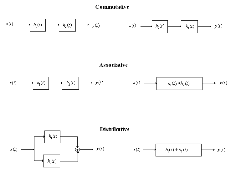
Convolution properties

Convolution satisfies the following three properties (see [link] ):

  • Commutative property
x ( t ) h ( t ) = h ( t ) x ( t ) size 12{x \( t \) * h \( t \) =h \( t \) * x \( t \) } {}
  • Associative property
x ( t ) h 1 ( t ) h 2 ( t ) = x ( t ) { h 1 ( t ) h 2 ( t ) } size 12{x \( t \) * h rSub { size 8{1} } \( t \) * h rSub { size 8{2} } \( t \) =x \( t \) * lbrace h rSub { size 8{1} } \( t \) * h rSub { size 8{2} } \( t \) rbrace } {}
  • Distributive property
x ( t ) { h 1 ( t ) + h 2 ( t ) } = x ( t ) h 1 ( t ) + x ( t ) h 2 ( t ) size 12{x \( t \) * lbrace h rSub { size 8{1} } \( t \) +h rSub { size 8{2} } \( t \) rbrace =x \( t \) * h rSub { size 8{1} } \( t \) +x \( t \) * h rSub { size 8{2} } \( t \) } {}
Convolution Properties

Get Jobilize Job Search Mobile App in your pocket Now!

Get it on Google Play Download on the App Store Now


Source:  OpenStax, An interactive approach to signals and systems laboratory. OpenStax CNX. Sep 06, 2012 Download for free at http://cnx.org/content/col10667/1.14
Google Play and the Google Play logo are trademarks of Google Inc.

Notification Switch

Would you like to follow the 'An interactive approach to signals and systems laboratory' conversation and receive update notifications?

Ask