Chapter 2: transformers  (Page 2/6)

Figure 2.4 Transformer with open secondary.

• The primary and secondary windings are actually interleaved in practice.
• A small steady-state current $i_{\varphi }$ (the exciting current) flows in the primary and establishes an alternating flux in the magnetic current.
• $e_1$ = emf induced in the primary (counter emf)

${\lambda }_1$ = flux linkage of the primary winding

$\varphi$ = flux in the core linking both windings

$N_1$ = number of turns in the primary winding

• The induced emf (counter emf) leads the flux by ${\text{90}}^o$

$e_1=\frac{{\mathrm{d\lambda }}_1}{\text{dt}}=N_1\frac{\mathrm{d\varphi }}{\text{dt}}$ (2.1)

$v_1=R_1{i}_{\varphi }+e_1$ (2.2)

• $e_1\approx v_1$ if the no-load resistance drop is very small and the waveforms of voltage and flux are very nearly sinusoidal.

$\varphi ={\phi }_{\text{max}}\text{sin}\mathrm{\omega t}$ (2.3)

$e_1=N_1\frac{\mathrm{d\varphi }}{\text{dt}}={\text{ωφ}}_{\text{max}}\text{cos}\mathrm{\omega t}$ (2.4)

$E_1=\frac{\mathrm{2\pi }}{\sqrt{2}}{\text{fN}}_1{\phi }_{\text{max}}=\sqrt{2}\pi {\text{fN}}_1{\phi }_{\text{max}}$ (2.5)

${\phi }_{\text{max}}=\frac{V_1}{\sqrt{2}\pi {\text{fN}}_1}$ (2.6)

• The core flux is determined by the applied voltage, its frequency, and the number of turns in the winding. The core flux is fixed by the applied voltage, and the required exciting current is determined by the magnetic properties of the core; the exciting current must adjust itself so as to produce the mmf required to create the flux demanded by (2.6).
• A curve of the exciting current as a function of time can be found graphically from the ac hysteresis loop as shown in Fig. 2.5.

Figure 2.5 Excitation phenomena. (a) Voltage, flux, and exciting current;

(b) corresponding hysteresis loop.

• If the exciting current is analyzed by Fourier-series methods, its is found to consist of a fundamental component and a series of odd harmonics.

• The fundamental component can, in turn, be resolved into two components, one in phase with the counter emf and the other lagging the counter emf by 90o.
  • Core-loss component: the in-phase component supplies the power absorbed by hysteresis and eddy-current losses in the core.
  • Magnetizing current: It comprises a fundamental component lagging the counter emf by ${\text{90}}^o$ , together with all the harmonics, of which the principal is the third (typically 40%).
• The peculiarities of the exciting-current waveform usually need not by taken into account, because the exciting current itself is small, especially in large transformers. (typically about 1 to 2 percent of full-load current)
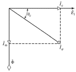
• Phasor diagram in Fig. 2.6.

${\hat{E}}_1=$ the rms value of the induced emf

$\hat{\Phi }=$ the rms value of the flux

${\hat{I}}_{\varphi }=$ the rms value of the equivalent sinusoidal exciting current

• $I_{\varphi }$ lags $E_1$ by a phase angle ${\theta }_c$ .

Figure 2.6 No-load phasor diagram.

• The core loss $P_c$ equals the product of the in-phase components of the ${\hat{E}}_1$ and $I_{\varphi }$ :

$P_c=E_1{I}_{\varphi }\text{cos}{\theta }_c$ (2.7)

• $I_c=$ core-loss current, $I_m=$ magnetizing current

§2.3 Effect of Secondary Current; Ideal Transformer

Figure 2.7 Ideal transformer and load.

• Ideal Transformer (Fig. 2.7)

• Assumptions:

1. Winding resistances are negligible.
2. Leakage flux is assumed negligible.
3. There are no losses in the core.
4. Only a negligible mmf is required to establish the flux in the core.

• The impressed voltage, the counter emf, the induced emf, and the terminal voltage:

$v_1=e_1=N_1\frac{\mathrm{d\varphi }}{\text{dt}}$ (2.8)

$v_2=e_2=N_2\frac{\mathrm{d\varphi }}{\text{dt}}$ (2.9)

$\frac{v_1}{v_2}=\frac{N_1}{N_2}$ (2.10)

• • An ideal transformer transforms voltages in the direct ratio of the turns in its windings.
• Let a load be connected to the secondary.