

| << Chapter < Page | Chapter >> Page > |
In
"Complex Numbers" , you learn that complex variables can be represented as points in the plane. MATLAB makes it easy for you to plot complex variables in a graph. Type. The graph window should be activated and the pointdisplayed by a 'o'. You must specify the symbol for display, and the authorized symbols for point display areand. When you are displaying a curve (to come later), no type is necessary. MATLAB automatically adjusts the scale on a graph to accommodate the value of the point being plotted. In this case, the range is
for the real part and
for the imaginary part.
'*'
Let's now plot a second complex number by typing. Note that the secondcommand erases the firstand changes the scaling to
and
. Sometimes you may want to have the points plotted on the same graph. To achieve this, you have to use the command hold on after the first plot. Try the following:
plot
The advantage in using thecommand is that there is no limit to the number of plot commands you can type before the hold is turned off, and
these plots may involve the same variable plotted over a range of values. You can also use different point displays. A disadvantage of thecommand is that the scaling is enforced by the first plot and is not adjusted for subsequent plots. This is why we plot the pointfirst. Try reversing the order of the plots and see what happens. This means that points outside the scaling will not be displayed. The commandpermits erasing the current graph for the nextcommand.
plot
You can freeze the scaling of the graph by using the command. MATLAB gives you the message
axis
This freezes the current axis scaling for subsequent plots. Similarly, if you type axis a second time, MATLAB resumes the automatic scaling feature and prints the message
The axis scaling can also be manually enforced by using the command
whereis the lower left corner andis the upper
right corner of the graph. This scaling remains in effect until the nextcommand is entered (with or without arguments).
axis
Another way to plot several complex numbers on the same graph is
to display them as a curve. For this purpose, you have to store the numbersin a vector. For example, type. Note that
the two points are at the two extremes of the line plotted on the graph. Ifyou specify a symbol, then no line is drawn, just the extreme points. Try.
plot(z,'o')
If you examine your current graph carefully, you will notice that the
unit lengths on the
x and
y axes are not quite the same. In fact, MATLAB
adjusts the length of an axis to conform to the overall size of the graph window.What this means is that a
45
o line will actually be displayed at an angle
depending on the overall aspect ratio of the graph window. To ensure thatthe aspect ratio is equal to 1, you may enter the command.
MATLAB will then enforce an aspect ratio equal to 1, regardless of the aspectratio for the outside graph window. This ensures that circles appear as circles
and not as ellipses. MATLAB will make the square graph as large as possibleto fit within the graph window. To go back to the default ratio, just type in.
axis('normal')
To add labels to your graph, the functions,, andare useful and self-explanatory. The argumentcontains a string of characters. Add the labelon the horizontal axis and the labelon the vertical axis of your graph. The commanddraws a grid on your graph. The grid does not remain in effect for the next plots. Try it.
grid
The plot Instruction. The plot instruction in MATLAB is very
versatile. It can be used to plot several different types of data. Its syntax isor. The
instruction will plot a vector of data versus another vector of data. The firstvector is referenced to the horizontal axis and the second to the vertical axis.
If only one vector is used, then it is plotted with reference to the verticalaxis while the horizontal axis is automatically forced to be the index of the
vector for the corresponding data point. The notation inside the apostrophesis optionally used to designate whether each element of the vector is to be
plotted as a single point with a certain symbol or as a curve with a straightline drawn between each data value. The colors can also be specified. Possible symbols are, and colors are(red, green, blue, and
white). Complex valued vectors are plotted by making the horizontal axis thereal part of the vector and the vertical axis the imaginary part. Warning: A
complex valued vector will automatically be plotted correctly on the complexplane (instead of real versus imaginary)
only if every element of the vector is complex valued. Try,,,and,to
clarify your understanding of plot. Use
.
plot (Real (z), Imag (z),'*')
We may summarize as follows:
plot(x,'*r') |
(red star—points with the values ofon vertical and indicies on horizontal)
x |
plot(y) |
(line—connected curve of the value ofon vertical and the value ofon horizontal)
x |
plot(x,y,'og') |
(line—connected curve of the value ofon vertical and the value ofon horizontal)
x |
plot(x,y,'og') |
(circle—points of the value ofon vertical and the value ofon horizontal)
x |
plot(real(z),imag(z)) |
(line—connectedplot ofon the complex plane)
z |
plot(real(z),imag(z),'+b') |
(blue plus—points ofon the complex plane).
z |
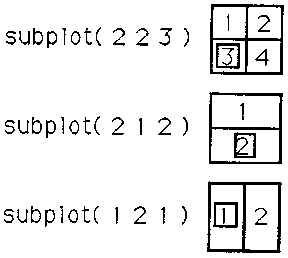
Subplots. It is possible to split the graphics screen up into several
separate smaller graphs rather than just one large graph. As many as foursubplots can be created. The MATLAB instructionsignifies
which of the smaller graphs is to be accessed with the next plot statement.The mnp argument consists of three digits. Theandare the numbers of
rows () and columns () into which the screen should be divided. Thedesignates which of the matrix elements is to be used. For example,
p
Help and Demos. MATLAB has on-line help and a collection of demonstrations. For a list of available functions, type
For help on a specific function,for example, type
sin
To learn how to use colon (;, a very important and versatile character) in MATLAB, type
The demos will also help you become more familiar with MATLAB and its capabilities. To run them, type
Notification Switch
Would you like to follow the 'A first course in electrical and computer engineering' conversation and receive update notifications?

|
|

|
|

|
|

|
|

|
|

|
|

|
|

|
|
|
|
|

|