

| << Chapter < Page | Chapter >> Page > |
Statistics students believe that the mean score on the first statistics test is 65. A statistics instructor thinks the mean score is higher than 65. He samples ten statistics students and obtains the scores
Set up the hypothesis test:
A 5% level of significance means that α = 0.05. This is a test of a single population mean .
H 0 : μ = 65 H a : μ >65
Since the instructor thinks the average score is higher, use a ">". The ">" means the test is right-tailed.
Determine the distribution needed:
Random variable: = average score on the first statistics test.
Distribution for the test: If you read the problem carefully, you will notice that there is no population standard deviation given . You are only given n = 10 sample data values. Notice also that the data come from a normal distribution. This means that the distribution for the test is a student's t .
Use t df . Therefore, the distribution for the test is t 9 where n = 10 and df = 10 - 1 = 9.
Calculate the p -value using the Student's t -distribution:
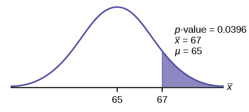
p -value = P ( >67) = 0.0396 where the sample mean and sample standard deviation are calculated as 67 and 3.1972 from the data.
Interpretation of the p -value: If the null hypothesis is true, then there is a 0.0396 probability (3.96%) that the sample mean is 65 or more.
Compare α and the p -value:
Since α = 0.05 and p -value = 0.0396. α > p -value.
Make a decision: Since α > p -value, reject H 0 .
This means you reject μ = 65. In other words, you believe the average test score is more than 65.
Conclusion: At a 5% level of significance, the sample data show sufficient evidence that the mean (average) test score is more than 65, just as the math instructor thinks.
The p -value can easily be calculated.
It is believed that a stock price for a particular company will grow at a rate of $5 per week with a standard deviation of $1. An investor believes the stock won’t grow as quickly. The changes in stock price is recorded for ten weeks and are as follows: $4, $3, $2, $3, $1, $7, $2, $1, $1, $2. Perform a hypothesis test using a 5% level of significance. State the null and alternative hypotheses, find the p -value, state your conclusion, and identify the Type I and Type II errors.
H 0 : μ = 5
H a : μ <5
p = 0.0082
Because p < α , we reject the null hypothesis. There is sufficient evidence to suggest that the stock price of the company grows at a rate less than $5 a week.
Type I Error: To conclude that the stock price is growing slower than $5 a week when, in fact, the stock price is growing at $5 a week (reject the null hypothesis when the null hypothesis is true).
Type II Error: To conclude that the stock price is growing at a rate of $5 a week when, in fact, the stock price is growing slower than $5 a week (do not reject the null hypothesis when the null hypothesis is false).
Joon believes that 50% of first-time brides in the United States are younger than their grooms. She performs a hypothesis test to determine if the percentage is the same or different from 50% . Joon samples 100 first-time brides and 53 reply that they are younger than their grooms. For the hypothesis test, she uses a 1% level of significance.
Set up the hypothesis test:
The 1% level of significance means that α = 0.01. This is a test of a single population proportion .
H 0 : p = 0.50 H a : p ≠ 0.50
The words "is the same or different from" tell you this is a two-tailed test.
Calculate the distribution needed:
Random variable: P′ = the percent of of first-time brides who are younger than their grooms.
Distribution for the test: The problem contains no mention of a mean. The information is given in terms of percentages. Use the distribution for P′ , the estimated proportion.
Therefore,
where p = 0.50, q = 1− p = 0.50, and n = 100
Calculate the p -value using the normal distribution for proportions:
p -value = P ( p′ <0.47 or p′ >0.53) = 0.5485
where x = 53, p′ = = 0.53.
Interpretation of the p -value: If the null hypothesis is true, there is 0.5485 probability (54.85%) that the sample (estimated) proportion is 0.53 or more OR 0.47 or less (see the graph in [link] ).
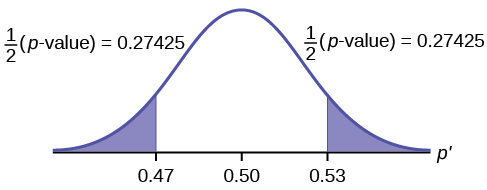
μ = p = 0.50 comes from H 0 , the null hypothesis.
p′ = 0.53. Since the curve is symmetrical and the test is two-tailed, the p′ for the left tail is equal to 0.50 – 0.03 = 0.47 where μ = p = 0.50. (0.03 is the difference between 0.53 and 0.50.)
Compare α and the p -value:
Since α = 0.01 and p -value = 0.5485. α < p -value.
Make a decision: Since α < p -value, you cannot reject H 0 .
Conclusion: At the 1% level of significance, the sample data do not show sufficient evidence that the percentage of first-time brides who are younger than their grooms is different from 50%.
The p -value can easily be calculated.
The Type I and Type II errors are as follows:
The Type I error is to conclude that the proportion of first-time brides who are younger than their grooms is different from 50% when, in fact, the proportion is actually 50%. (Reject the null hypothesis when the null hypothesis is true).
The Type II error is there is not enough evidence to conclude that the proportion of first time brides who are younger than their grooms differs from 50% when, in fact, the proportion does differ from 50%. (Do not reject the null hypothesis when the null hypothesis is false.)
Notification Switch
Would you like to follow the 'Statistics i - math1020 - red river college - version 2015 revision a - draft 2015-10-24' conversation and receive update notifications?

|
|

|
|

|
|

|
|

|
|

|
|
|
|
|

|
|
|
|
|

|