<< Chapter < Page Chapter >> Page >
This module is part of the collection, A First Course in Electrical and Computer Engineering . The LaTeX source files for this collection were created using an optical character recognition technology, and because of this process there may be more errors than usual. Please contact us if you discover any errors.

When we design a filter, we design it for a purpose. For example, a moving average filter is often designed to pass relatively constant data whileaveraging out relatively variable data. In an effort to clarify the behavior of a filter, we typically analyze its response to a standard set of test signals. Wewill call the impulse , the step , and the complex exponential the standard test signals.

Unit Pulse Sequence. The unit pulse sequence is the sequence

u n = δ n = 1 , n = 0 0 , n 0 .

This sequence, illustrated in Figure 1 , consists of all zeros except for a single one at n = 0 . If the unit pulse sequence is passed through a moving average filter (whether finite or not), then the output is called the unit pulse response :
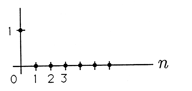
h n = k = 0 w k δ n - k = w n .
This Cartesian graph is relatively simple. The positive portion of the x axis is marked with dashed dots spaced equidistant from each other. The first three are labeled 1, 2, and 3. There are three more dots to the right of those dots. The x axis is labeled n. The y axis only has one dashed point and the it is labeled 1. This Cartesian graph is relatively simple. The positive portion of the x axis is marked with dashed dots spaced equidistant from each other. The first three are labeled 1, 2, and 3. There are three more dots to the right of those dots. The x axis is labeled n. The y axis only has one dashed point and the it is labeled 1.
Unit Pulse Sequence

(Note that δ n - k = 0 unless n = k . ) So the unit pulse sequence may be used to read out the weights of a moving average filter. It is common practice to use w k (the k t h weight) and h k (the k t h impulse response) interchangeably.

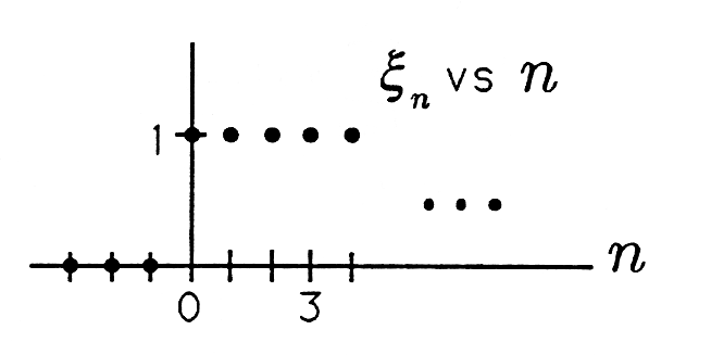
Unit Step Sequence. The unit step sequence is the sequence

u n = ξ n = 1 , n 0 0 , n < 0 .

This sequence is illustrated in Figure 2 . When this sequence is applied to a moving average filter, the result is the unit step response

g n = k = 0 n w k = k = 0 n h k .

The unit step response is just the sequence of partial sums of the unit pulse response.

This Cartesian graph has three dashed dots on the negative portion of the x acis. The origin is labeled 0. On the poisitive side of the x axis there are four dashes. The third dash is labeled 3 and the x axis is labeled n. On the positive portion of the y-axis there is a single dashed dot labeled 1. To the right of this dashed dot there are four dots that are directly above the dashes on the positive portion of the x axis. Just above and to the right of the dots is the expression ξ_n vs n. Directly below this this symbol are three more dots. These dots are slightly above and to the right of the dashes on the x axis. This Cartesian graph has three dashed dots on the negative portion of the x acis. The origin is labeled 0. On the poisitive side of the x axis there are four dashes. The third dash is labeled 3 and the x axis is labeled n. On the positive portion of the y-axis there is a single dashed dot labeled 1. To the right of this dashed dot there are four dots that are directly above the dashes on the positive portion of the x axis. Just above and to the right of the dots is the expression ξ_n vs n. Directly below this this symbol are three more dots. These dots are slightly above and to the right of the dashes on the x axis.
Unit Step Sequence

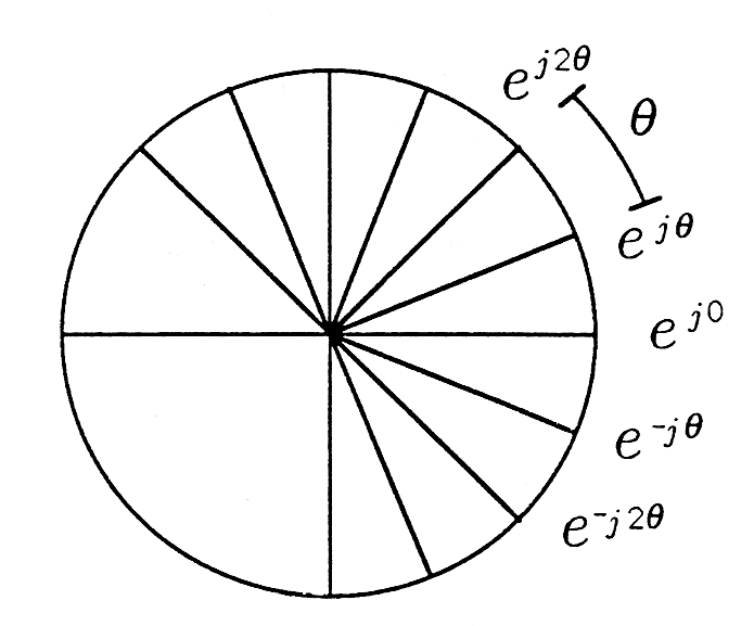
Complex Exponential Sequence. The complex exponential sequence is the sequence

u k = e j k θ , k = 0 , ± 1 , ± 2 , ...

This sequence, illustrated in Figure 3 , is a “discrete-time phasor” that “ratchets” counterclockwise (CCW) as k moves to k + 1 and clockwise (CW) as k moves to k - 1 . Each time the phasor ratchets, it turns out an angle of θ . Why should such a sequence be a useful test sequence? There are two reasons.

This is a circle divided in to many slices. The bottom left is the size of a quarter of the circle. Above this section is a 1/8th sized portion and the rest of the circle is divided into 1/16th sized portions. The right half of the circle has mathematical expression associated with the different slices. The second slice from the top is labeled e^{j2θ} the next slice has an arch capped on either end with horizontal lines and the actual arch is labeled θ. The next few slices proceeding down are labeled e^{jθ}, then e^{j0}, then e^{-jθ}, and finally e^{-j2θ}. This is a circle divided in to many slices. The bottom left is the size of a quarter of the circle. Above this section is a 1/8th sized portion and the rest of the circle is divided into 1/16th sized portions. The right half of the circle has mathematical expression associated with the different slices. The second slice from the top is labeled e^{j2θ} the next slice has an arch capped on either end with horizontal lines and the actual arch is labeled θ. The next few slices proceeding down are labeled e^{jθ}, then e^{j0}, then e^{-jθ}, and finally e^{-j2θ}.
Discrete-Time Phasor

(i) e j k θ represents (or codes) cos k θ . The real part of the sequence e j k θ is the cosinusoidal sequence cos k θ :

Re [ e j k θ ] = cos k θ .

Therefore the discrete-time phasor e j k θ represents (or codes) cos k θ in the same way that the continuous-time phasor e j ω t codes cos ω t . If the moving average filter

x n = k = 0 h k u n - k

has real coefficients, we can get the response to a cosinusoidal sequence by taking the real part of the following sum:

x n = k = 0 h k cos ( n - k ) θ = Re [ k = 0 h k e j ( n - k ) θ ] = Re [ e j n θ k = 0 h k e - j k θ ] .

In this formula, the sum

k = 0 h k e - j k θ

is called the complex frequency response of the filter and is given the symbol

H ( e j θ ) = k = 0 h k e - j k θ .

This complex frequency response is just a complex number, with a magnitude | H ( e j θ ) | and a phase arg H ( e j θ ) . Therefore the output of the moving average filter is

x n = Re [ e j n θ H ( e j θ ) ] = Re [ e j n θ | H ( e j θ ) | e j arg H ( e j θ ) ] = | H ( e j θ ) | c o s [ n θ + arg H ( e j θ ) ] .

This remarkable result says that the output is also cosinusoidal, but its amplitude is | H ( e j θ ) | rather than 1, and its phase is a r g H ( e j θ ) rather than 0. In the examples to follow, we will show that the complex “gain” H ( e j θ ) can be highly selective in θ , meaning that cosines of some angular frequencies are passed with little attenuation while cosines of other frequencies are dramatically attenuated. By choosing the filter coefficients, we can design the frequency selectivity we would like to have.

(ii) e j k θ is a sampled data version of e j ω t . The discrete-time phasor e j k θ can be produced physically by sampling the continuous-time phasor e j ω t at the periodic sampling instants t k = k T :

e j k θ = e j ω t | t = k T = e j ω k T θ = ω T .

The dimensions of θ are radians, the dimensions of ω are radians/second, and the dimensions of T are seconds. We call T the sampling interval and 1 T the sampling rate or sampling frequency. If the original angular frequency of thephasor e j ω t is increased to ω + m ( 2 π T ) , then the discrete-time phasor remains e j k θ :

e j [ ω + m ( 2 π / T ) ] t | t = k T = e j ( ω k T + k m 2 π ) = e j k θ .

This means that all continuous-time phasors of the form e j [ ω + m ( 2 π / T ) ] t “hide under the same alias” when viewed through the sampling operation. Thatis, the sampled-data phasor cannot distinguish the frequency ω from the frequency ω + m 2 π T . In your subsequent courses you will study aliasing in more detail and study the Nyquist rule for sampling:

T 2 π Ω ; 1 T Ω 2 π

This rule says that you must sample signals at a rate ( 1 T ) that exceeds the bandwidth Ω 2 π of the signal.

Let's pass the cosinusoidal sequence u k = cos k θ through the finite moving average filter

x n = k = 0 N - 1 h k u n - k h k = 1 N k = 0 , 1 , ... , N - 1 .

We know from our previous result that the output is

x n = | H ( e j θ ) | cos [ n θ + arg H ( e j θ ) ] .

The complex frequency response for this example is

H ( e j θ ) = k = 0 N - 1 1 N e - j k θ = 1 N 1 - e - j N θ 1 - e - j θ

(Do you see your old friend, the finite sum formula, at work?) Let's try to manipulate the result into a more elegant form:

H ( e j θ ) = 1 N e - j ( N / 2 ) θ [ e j ( N / 2 ) θ - e - j ( N / 2 ) θ ] e - j ( θ / 2 ) [ e j ( θ / 2 ) - e - j ( θ / 2 ) ] = 1 N e - j [ ( N - 1 ) / 2 ] θ sin ( N 2 θ ) sin ( 1 2 θ ) .

The magnitude of the function H ( e j θ ) is

| H ( e j θ ) | = 1 N , | sin ( N 2 θ ) sin ( 1 2 θ ) | .

At θ = 0 , corresponding to a “DC phasor,” H ( e j θ ) equals 1; at θ = 2 π N | H ( e j θ ) = 0 | . The magnitude of the complex frequency response is plotted in Figure 4 .

This Cartesian graph contains a series of arches progressing along the x axis. The first arch starts at the far left end of the negative portion of the x axis and returns to the x axis about halfway to the origin. This point is labeled -2π/N. The next arch begins at this same point and returns to the x axis the same distance away from the origin as it left  but now on the positive side of the x axis. This point is labeled 2π/N. At about the peak of this arch on the negative side of the x axis is the mark 1. The third arch begins at point 2π/N and ends at a point labeled 2(2π/N). There is one final arch that starts at the last point and an unlabeled point. The x axis is labeled θ. This Cartesian graph contains a series of arches progressing along the x axis. The first arch starts at the far left end of the negative portion of the x axis and returns to the x axis about halfway to the origin. This point is labeled -2π/N. The next arch begins at this same point and returns to the x axis the same distance away from the origin as it left  but now on the positive side of the x axis. This point is labeled 2π/N. At about the peak of this arch on the negative side of the x axis is the mark 1. The third arch begins at point 2π/N and ends at a point labeled 2(2π/N). There is one final arch that starts at the last point and an unlabeled point. The x axis is labeled θ.
Frequency Selectivity of a Moving Average Filter

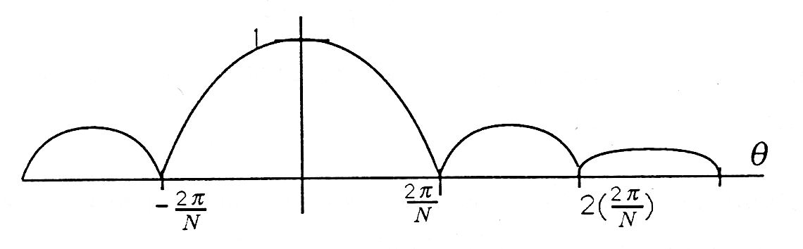
This result shows that the moving average filter is frequency selective, passing low frequencies with gain near 1 and high frequencies with gain near 0.

Get Jobilize Job Search Mobile App in your pocket Now!

Get it on Google Play Download on the App Store Now


Source:  OpenStax, A first course in electrical and computer engineering. OpenStax CNX. Sep 14, 2009 Download for free at http://cnx.org/content/col10685/1.2
Google Play and the Google Play logo are trademarks of Google Inc.

Notification Switch

Would you like to follow the 'A first course in electrical and computer engineering' conversation and receive update notifications?

Ask