

| << Chapter < Page | Chapter >> Page > |
The size of these income and substitution effects will differ from person to person, depending on individual preferences. For example, if Ogden’s substitution effect away from pizza and toward haircuts is especially strong, and outweighs the income effect, then a higher price for pizza might lead to increased consumption of haircuts. This case would be drawn on the graph so that the point of tangency between the new budget constraint and the relevant indifference curve occurred below point B and to the right. Conversely, if the substitution effect away from pizza and toward haircuts is not as strong, and the income effect on is relatively stronger, then Ogden will be more likely to react to the higher price of pizza by consuming less of both goods. In this case, his optimal choice after the price change will be above and to the left of choice B on the new budget constraint.
Although the substitution and income effects are often discussed as a sequence of events, it should be remembered that they are twin components of a single cause—a change in price. Although you can analyze them separately, the two effects are always proceeding hand in hand, happening at the same time.
Indifference curves provide an analytical tool for looking at all the choices that provide a single level of utility. They eliminate any need for placing numerical values on utility and help to illuminate the process of making utility-maximizing decisions. They also provide the basis for a more detailed investigation of the complementary motivations that arise in response to a change in a price, wage or rate of return—namely, the substitution and income effects.
If you are finding it a little tricky to sketch diagrams that show substitution and income effects so that the points of tangency all come out correctly, it may be useful to follow this procedure.
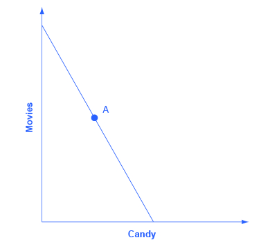
Step 1. Begin with a budget constraint showing the choice between two goods, which this example will call “candy” and “movies.” Choose a point A which will be the optimal choice, where the indifference curve will be tangent—but it is often easier not to draw in the indifference curve just yet. See [link] .
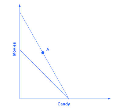
Step 2. Now the price of movies changes: let’s say that it rises. That shifts the budget set inward. You know that the higher price will push the decision-maker down to a lower level of utility, represented by a lower indifference curve. But at this stage, draw only the new budget set. See [link] .
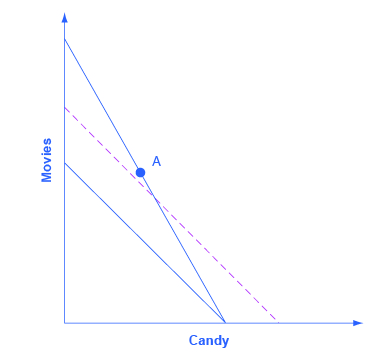
Step 3. The key tool in distinguishing between substitution and income effects is to insert a dashed line, parallel to the new budget line. This line is a graphical tool that allows you to distinguish between the two changes: (1) the effect on consumption of the two goods of the shift in prices—with the level of utility remaining unchanged—which is the substitution effect; and (2) the effect on consumption of the two goods of shifting from one indifference curve to the other—with relative prices staying unchanged—which is the income effect. The dashed line is inserted in this step. The trick is to have the dashed line travel close to the original choice A, but not directly through point A. See [link] .
Step 4. Now, draw the original indifference curve, so that it is tangent to both point A on the original budget line and to a point C on the dashed line. Many students find it easiest to first select the tangency point C where the original indifference curve touches the dashed line, and then to draw the original indifference curve through A and C. The substitution effect is illustrated by the movement along the original indifference curve as prices change but the level of utility holds constant, from A to C. As expected, the substitution effect leads to less consumed of the good that is relatively more expensive, as shown by the “s” (substitution) arrow on the vertical axis, and more consumed of the good that is relatively less expensive, as shown by the “s” arrow on the horizontal axis. See [link] .
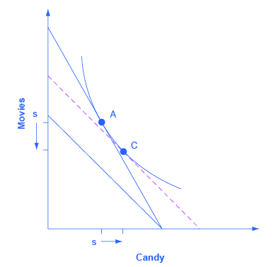
Step 5. With the substitution effect in place, now choose utility-maximizing point B on the new opportunity set. When you choose point B, think about whether you wish the substitution or the income effect to have a larger impact on the good (in this case, candy) on the horizontal axis. If you choose point B to be directly in a vertical line with point A (as is illustrated here), then the income effect will be exactly offsetting the substitution effect on the horizontal axis. If you insert point B so that it lies a little to right of the original point A, then the substitution effect will exceed the income effect. If you insert point B so that it lies a little to the left of point A, then the income effect will exceed the substitution effect. The income effect is the movement from C to B, showing how choices shifted as a result of the decline in buying power and the movement between two levels of utility, with relative prices remaining the same. With normal goods, the negative income effect means less consumed of each good, as shown by the direction of the “i” (income effect) arrows on the vertical and horizontal axes. See [link] .

In sketching substitution and income effect diagrams, you may wish to practice some of the following variations: (1) Price falls instead of a rising; (2) The price change affects the good on either the vertical or the horizontal axis; (3) Sketch these diagrams so that the substitution effect exceeds the income effect; the income effect exceeds the substitution effect; and the two effects are equal.
One final note: The helpful dashed line can be drawn tangent to the new indifference curve, and parallel to the original budget line, rather than tangent to the original indifference curve and parallel to the new budget line. Some students find this approach more intuitively clear. The answers you get about the direction and relative sizes of the substitution and income effects, however, should be the same.
Notification Switch
Would you like to follow the 'Openstax microeconomics in ten weeks' conversation and receive update notifications?

|
|

|
|

|
|

|
|

|
|

|
|

|
|
|
|
|

|
|

|