<< Chapter < Page Chapter >> Page >

Chapter opener: modeling a motorcycle suspension system

This picture is a shock absorber on a motorcycle.
(credit: modification of work by nSeika, Flickr)

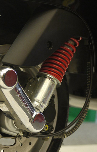
For motocross riders, the suspension systems on their motorcycles are very important. The off-road courses on which they ride often include jumps, and losing control of the motorcycle when they land could cost them the race.

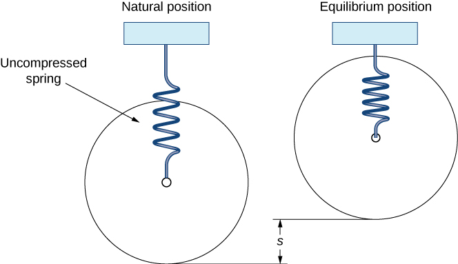
This suspension system can be modeled as a damped spring-mass system. We define our frame of reference with respect to the frame of the motorcycle. Assume the end of the shock absorber attached to the motorcycle frame is fixed. Then, the “mass” in our spring-mass system is the motorcycle wheel. We measure the position of the wheel with respect to the motorcycle frame. This may seem counterintuitive, since, in many cases, it is actually the motorcycle frame that moves, but this frame of reference preserves the development of the differential equation that was done earlier. As with earlier development, we define the downward direction to be positive.

When the motorcycle is lifted by its frame, the wheel hangs freely and the spring is uncompressed. This is the spring’s natural position. When the motorcycle is placed on the ground and the rider mounts the motorcycle, the spring compresses and the system is in the equilibrium position ( [link] ).

This figure has two springs attached above at a fixed point. The first spring is labeled, “Natural Position,” and has an uncompressed spring hanging vertically. The second spring is labeled, “Equilibrium Position,” and has a compressed spring hanging vertically. The vertical difference between the two springs is labeled, “s.”
We can use a spring-mass system to model a motorcycle suspension.

This system can be modeled using the same differential equation we used before:

m x + b x + k x = 0 .

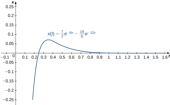
A motocross motorcycle weighs 204 lb, and we assume a rider weight of 180 lb. When the rider mounts the motorcycle, the suspension compresses 4 in., then comes to rest at equilibrium. The suspension system provides damping equal to 240 times the instantaneous vertical velocity of the motorcycle (and rider).

  1. Set up the differential equation that models the behavior of the motorcycle suspension system.
  2. We are interested in what happens when the motorcycle lands after taking a jump. Let time t = 0 denote the time when the motorcycle first contacts the ground. If the motorcycle hits the ground with a velocity of 10 ft/sec downward, find the equation of motion of the motorcycle after the jump.
  3. Graph the equation of motion over the first second after the motorcycle hits the ground.
  1. We have defined equilibrium to be the point where m g = k s , so we have
    m g = k s 384 = k ( 1 3 ) k = 1152 .

    We also have
    W = m g 384 = m ( 32 ) m = 12 .

    Therefore, the differential equation that models the behavior of the motorcycle suspension is
    12 x + 240 x + 1152 x = 0 .

    Dividing through by 12, we get
    x + 20 x + 96 x = 0 .
  2. The differential equation found in part a. has the general solution
    x ( t ) = c 1 e −8 t + c 2 e −12 t .

    Now, to determine our initial conditions, we consider the position and velocity of the motorcycle wheel when the wheel first contacts the ground. Since the motorcycle was in the air prior to contacting the ground, the wheel was hanging freely and the spring was uncompressed. Therefore the wheel is 4 in. ( 1 3 ft ) below the equilibrium position (with respect to the motorcycle frame), and we have x ( 0 ) = 1 3 . According to the problem statement, the motorcycle has a velocity of 10 ft/sec downward when the motorcycle contacts the ground, so x ( 0 ) = 10 . Applying these initial conditions, we get c 1 = 7 2 and c 2 = ( 19 6 ) , so the equation of motion is
    x ( t ) = 7 2 e −8 t 19 6 e −12 t .
  3. The graph is shown in [link] .
    This figure is the graph of the function f(x) = 7/2e^−8t −19/6e^−12t.  The vertical axis is scaled in increments of 0.05, and the horizontal axis is labeled, “t.” It is scaled in increments of tenths. The graph intersects the horizontal axis increasing, reaches a maximum, then decreases. The horizontal axis is a horizontal asymptote.
    Graph of the equation of motion over a time of one second.
Got questions? Get instant answers now!
Practice Key Terms 3

Get Jobilize Job Search Mobile App in your pocket Now!

Get it on Google Play Download on the App Store Now


Source:  OpenStax, Calculus volume 3. OpenStax CNX. Feb 05, 2016 Download for free at http://legacy.cnx.org/content/col11966/1.2
Google Play and the Google Play logo are trademarks of Google Inc.

Notification Switch

Would you like to follow the 'Calculus volume 3' conversation and receive update notifications?

Ask