7.1 Second-order linear equations  (Page 7/15)

Initial-value problems and boundary-value problems

So far, we have been finding general solutions to differential equations. However, differential equations are often used to describe physical systems, and the person studying that physical system usually knows something about the state of that system at one or more points in time. For example, if a constant-coefficient differential equation is representing how far a motorcycle shock absorber is compressed, we might know that the rider is sitting still on his motorcycle at the start of a race, time $t=t_0.$ This means the system is at equilibrium, so $y(t_0)=0,$ and the compression of the shock absorber is not changing, so $y^{\prime }(t_0)=0.$ With these two initial conditions and the general solution to the differential equation, we can find the specific solution to the differential equation that satisfies both initial conditions. This process is known as solving an initial-value problem . (Recall that we discussed initial-value problems in Introduction to Differential Equations .) Note that second-order equations have two arbitrary constants in the general solution, and therefore we require two initial conditions to find the solution to the initial-value problem.

Sometimes we know the condition of the system at two different times. For example, we might know $y(t_0)=y_0$ and $y(t_1)=y_1.$ These conditions are called boundary conditions    , and finding the solution to the differential equation that satisfies the boundary conditions is called solving a boundary-value problem    .

Mathematicians, scientists, and engineers are interested in understanding the conditions under which an initial-value problem or a boundary-value problem has a unique solution. Although a complete treatment of this topic is beyond the scope of this text, it is useful to know that, within the context of constant-coefficient, second-order equations, initial-value problems are guaranteed to have a unique solution as long as two initial conditions are provided. Boundary-value problems, however, are not as well behaved. Even when two boundary conditions are known, we may encounter boundary-value problems with unique solutions, many solutions, or no solution at all.

Solving an initial-value problem and graphing the solution

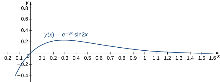
Solve the following initial-value problem and graph the solution:

$y\text{″}+6y^{\prime }+13y=0,y(0)=0,y^{\prime }(0)=2$

We already solved this differential equation in [link] b. and found the general solution to be

$y(x)=e^{\mathrm{-3}x}\left(c_1\text{cos}2x+c_2\text{sin}2x\right).$

Then

$y^{\prime }(x)=e^{\mathrm{-3}x}\left(\mathrm{-2}{c}_1\text{sin}2x+2c_2\text{cos}2x\right)-3e^{\mathrm{-3}x}\left(c_1\text{cos}2x+c_2\text{sin}2x\right).$

When $x=0,$ we have $y(0)=c_1$ and $y^{\prime }(0)=2c_2-3c_1.$ Applying the initial conditions, we obtain

$\begin{array}{ccc}\hfill c_1& =\hfill & 0\hfill \\ \hfill \mathrm{-3}{c}_1+2c_2& =\hfill & 2.\hfill \end{array}$

Therefore, $c_1=0,$ $c_2=1,$ and the solution to the initial value problem is shown in the following graph.

$y=e^{\mathrm{-3}x}\text{sin}2x\text{.}$

Got questions? Get instant answers now!

Got questions? Get instant answers now!