7.1 Lab 7: system response, analog and digital filters

Response of discrete-time systems

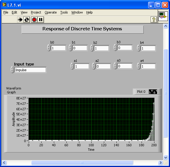
This lab involves analyzing the response of discrete-time systems. Responses are calculated for three different kinds of inputs; impulse, step and sine. [link] shows the completed block diagram. Connect the input variable w to an Enum Control so that an input type (impulse, step or sine) can be selected. The response of this system to any discrete-time input $x[n]$ can be written as

For this example, consider five b’s and four a’s. The system output is displayed using a waveform graph.

[link] shows the front panel of the above system. The front panel can be used to interactively select the input type and set the coefficients a and b. The system response for a particular type of input (impulse, step or sine) is shown in the waveform graph.

Square root

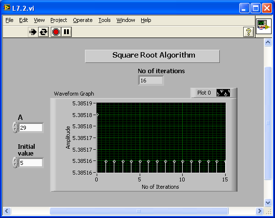
As another example of discrete-time systems, let us consider taking the square root of an integer number. Often computers and calculators compute the square root of a positive number $A$ using the following recursive equation:

If the input $x[n]$ to this equation is set as a step function of amplitude A, then $y[n]$ converges to the square root of A after several iterations.

[link] shows the block diagram for a square root computation system. The number of iterations required to converge to the true value is shown in the output. The initial condition Initial value is set as a control. [link] shows the corresponding front panel.

Analog and digital filtering

In this section, let us examine a basic analog and digital filtering example by implementing a lowpass and a highpass filter in the analog and digital domains, respectively. [link] shows the completed block diagram of the filtering system. For analog approximation of the signals, use a higher sampling rate (dw1=0.01). To detect whether the filtering is lowpass or highpass, use the Enum Control Analog filter type. Calculate the magnitude and phase response of these filters using equations provided in Chapter 7 for analog and digital filters. Set the values of R and C as controls, and display the responses using a Build Waveform function and a waveform graph.

For the digital case, use a lower sampling rate (dw2=0.001). With the Enum controls Digital filter type 1 and Digital filter type 2, select lowpass or highpass and FIR or IIR filter type. Use a Build Waveform function and a waveform graph to display the magnitude and phase responses of the digital filters. [link] shows the front panel of this filtering system. For a better view of magnitude response of the digital filter, set the properties of the waveform graph as shown in [link] .

Lab exercises

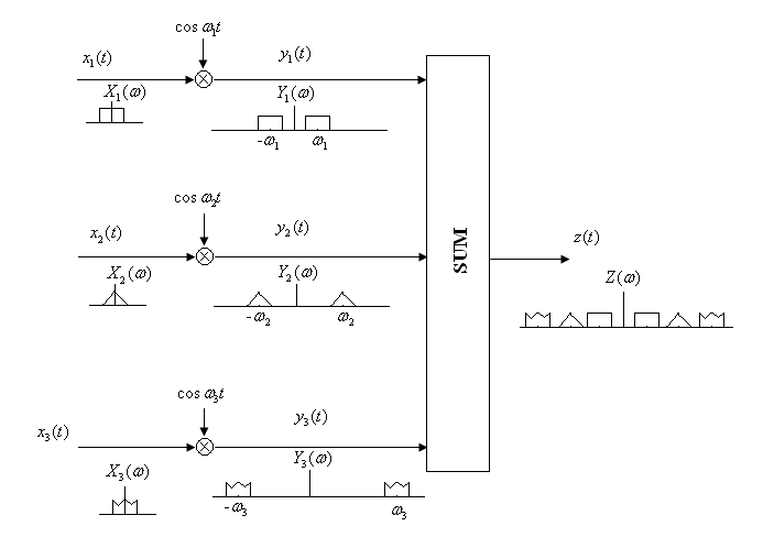
Frequency Division Multiplexing (FDM)

FDM is widely used in digital communication to simultaneously transmit multiple signals over a single wideband channel (for details, refer to [link] ). For FDM communication, individual signals are multiplied with different carriers to avoid overlaps in the frequency domain. Their time domain processing and corresponding frequency spectrums are shown in [link] . Build a VI to implement an FDM communication system for three signals $x_1(t),x_2(t)$ and $x_3(t)$ . Use the files echo_1.wav and firetrucksiren.wav on the book website and a random noise with a frequency range of 20 Hz to 20 kHz to serve as these signals.

Insert Solution Text Here

FDM Detector

Build a VI to implement an FDM detector system for detecting the signal $x_1(t)$ as shown in [link] .

Insert Solution Text Here